BIO 223L Notes, Fall 2011

BIOL 223 Genetics Laboratory Manual 2010-2011 Biology Department American University of Beirut Contributions by Layane Hajjar & Colin Smith Edited by Nadine Darwiche, Hana Ibrahim, & Colin Smith Coordinated by Hala Gali-Muhtasib Cover image: Drosophila melanogaster mitochondrial ND1 gene fragment with translations. 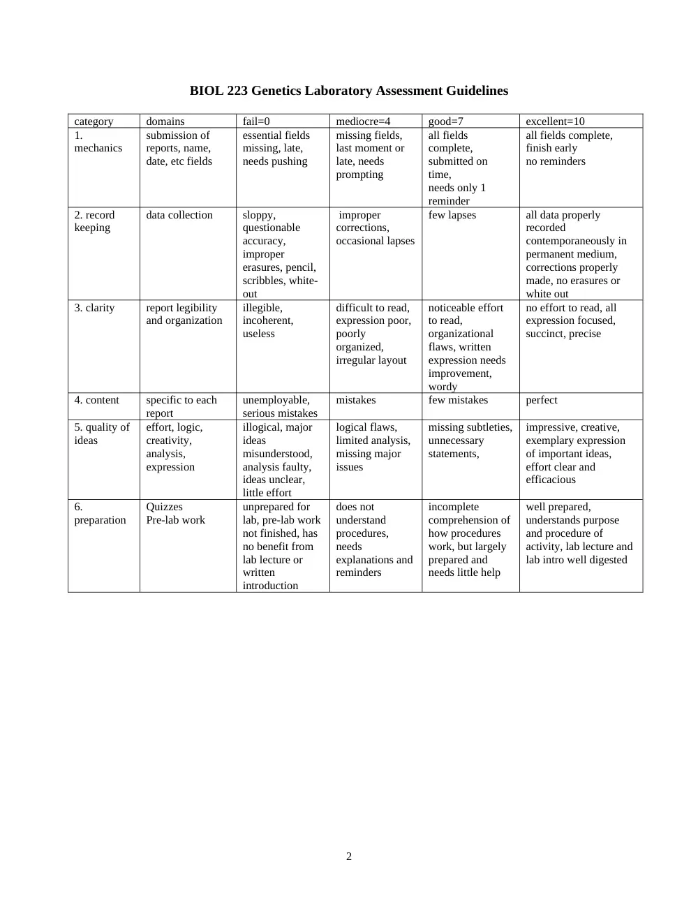Acknowledgments Jimmy Asraoui for assistance with dipteran phylogeny resources Khouzama Knio for Drosophila figures 1 BIOL 223 Genetics Laboratory Assessment Guidelines category domains fail=0 mediocre=4 good=7 excellent=10 1. mechanics submission of reports, name, date, etc fields essential fields missing, late, needs pushing missing fields, last moment or late, needs prompting all fields complete, submitted on time, needs only 1 reminder all fields complete, finish early no reminders 2. record keeping data collection sloppy, questionable accuracy, improper erasures, pencil, scribbles, white- out improper corrections, occasional lapses few lapses all data properly recorded contemporaneously in permanent medium, corrections properly made, no erasures or white out 3. clarity report legibility and organization illegible, incoherent, useless difficult to read, expression poor, poorly organized, irregular layout noticeable effort to read, organizational flaws, written expression needs improvement, wordy no effort to read, all expression focused, succinct, precise 4. content specific to each report unemployable, serious mistakes mistakes few mistakes perfect 5. quality of ideas effort, logic, creativity, analysis, expression illogical, major ideas misunderstood, analysis faulty, ideas unclear, little effort logical flaws, limited analysis, missing major issues missing subtleties, unnecessary statements, impressive, creative, exemplary expression of important ideas, effort clear and efficacious 6. 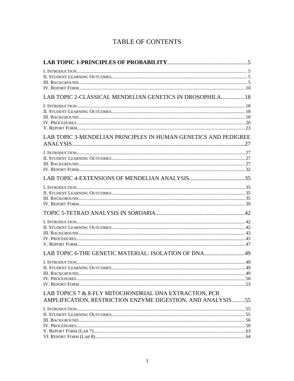preparation Quizzes Pre-lab work unprepared for lab, pre-lab work not finished, has no benefit from lab lecture or written introduction does not understand procedures, needs explanations and reminders incomplete comprehension of how procedures work, but largely prepared and needs little help well prepared, understands purpose and procedure of activity, lab lecture and lab intro well digested 2 TABLE OF CONTENTS LAB TOPIC 1-PRINCIPLES OF PROBABILITY.......................................................5 I. INTRODUCTION.............................................................................................................................................. 5 II. STUDENT LEARNING OUTCOMES.................................................................................................................5 III. BACKGROUND.............................................................................................................................................5 IV. REPORT FORM...........................................................................................................................................10 LAB TOPIC 2-CLASSICAL MENDELIAN GENETICS IN DROSOPHILA................18 I. INTRODUCTION............................................................................................................................................18 II. STUDENT LEARNING OUTCOMES...............................................................................................................18 III. BACKGROUND...........................................................................................................................................18 IV. PROCEDURES.............................................................................................................................................20 V. REPORT FORM............................................................................................................................................23 LAB TOPIC 3-MENDELIAN PRINCIPLES IN HUMAN GENETICS AND PEDIGREE ANALYSIS........................................................................................................................27 I. INTRODUCTION............................................................................................................................................27 II. STUDENT LEARNING OUTCOMES...............................................................................................................27 III. BACKGROUND...........................................................................................................................................27 IV. REPORT FORM...........................................................................................................................................32 LAB TOPIC 4-EXTENSIONS OF MENDELIAN ANALYSIS......................................35 I. INTRODUCTION............................................................................................................................................35 II. STUDENT LEARNING OUTCOMES...............................................................................................................35 III. BACKGROUND...........................................................................................................................................35 IV. REPORT FORM...........................................................................................................................................39 TOPIC 5-TETRAD ANALYSIS IN SORDARIA..............................................................42 I. INTRODUCTION............................................................................................................................................42 II. STUDENT LEARNING OUTCOMES...............................................................................................................42 III. BACKGROUND...........................................................................................................................................43 IV. PROCEDURES.............................................................................................................................................45 V. REPORT FORM............................................................................................................................................47 LAB TOPIC 6-THE GENETIC MATERIAL: ISOLATION OF DNA............................49 I. INTRODUCTION............................................................................................................................................49 II. STUDENT LEARNING OUTCOMES...............................................................................................................49 III. BACKGROUND...........................................................................................................................................49 IV. PROCEDURES.............................................................................................................................................50 IV. REPORT FORM...........................................................................................................................................53 LAB TOPICS 7 & 8-FLY MITOCHONDRIAL DNA EXTRACTION, PCR AMPLIFICATION, RESTRICTION ENZYME DIGESTION, AND ANALYSIS.........55 I. INTRODUCTION............................................................................................................................................55 II. STUDENT LEARNING OUTCOMES...............................................................................................................55 III. BACKGROUND...........................................................................................................................................56 IV. PROCEDURES.............................................................................................................................................59 V. REPORT FORM (LAB 7)..............................................................................................................................63 VI. 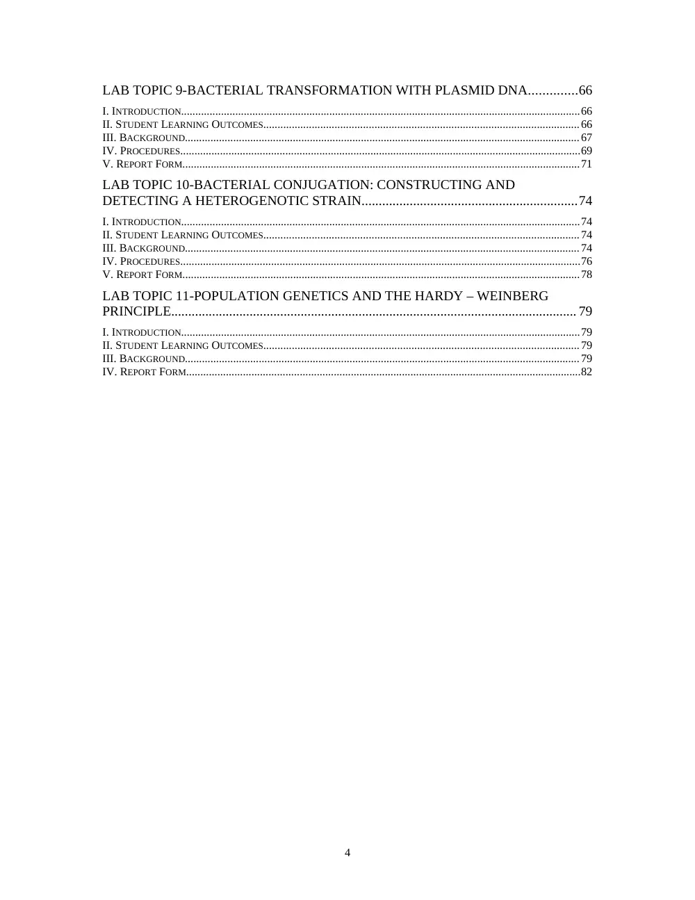REPORT FORM (LAB 8).............................................................................................................................64 3 LAB TOPIC 9-BACTERIAL TRANSFORMATION WITH PLASMID DNA..............66 I. INTRODUCTION............................................................................................................................................66 II. STUDENT LEARNING OUTCOMES...............................................................................................................66 III. BACKGROUND...........................................................................................................................................67 IV. PROCEDURES.............................................................................................................................................69 V. REPORT FORM............................................................................................................................................71 LAB TOPIC 10-BACTERIAL CONJUGATION: CONSTRUCTING AND DETECTING A HETEROGENOTIC STRAIN...............................................................74 I. INTRODUCTION............................................................................................................................................74 II. STUDENT LEARNING OUTCOMES...............................................................................................................74 III. BACKGROUND...........................................................................................................................................74 IV. PROCEDURES.............................................................................................................................................76 V. REPORT FORM............................................................................................................................................78 LAB TOPIC 11-POPULATION GENETICS AND THE HARDY – WEINBERG PRINCIPLE....................................................................................................................... 79 I. INTRODUCTION............................................................................................................................................79 II. STUDENT LEARNING OUTCOMES...............................................................................................................79 III. BACKGROUND...........................................................................................................................................79 IV. REPORT FORM...........................................................................................................................................82 4 Lab Topic 1 Lab Topic 1-Principles of Probability Colin Smith and Layane Hajjar I. Introduction The laws of probability can be used to predict the likelihood of chance events, where there is a limited number of outcomes. The coin toss is a simple example. When a coin is tossed into the air and allowed to come to rest, it may land showing either face, but the complexity of the toss makes it impossible to control or predict how it will land. For every toss, one of two faces will show: the obverse "heads" (H), or the reverse "tails" (T). The expectation is that for each toss, the two outcomes have equal probability, and that with sufficient tosses the observations will approach a limit of 0.5 H and 0.5 T. Similarly, when a cubic die is rolled, there is a 1/6 chance of arriving at any one of the six numbers marked on the different faces of the die. Statistical tests examine whether the difference between observations and expectations are likely due to chance, where the expectations derive from probability calculations of a theoretical model. In the first part of this laboratory exercise, you will examine a shaved die, conceive a hypothesis as to how its rolling will be altered, formulate a prediction to test your hypothesis, collect data, and apply statistical tests to find the probability your hypothesis is false. You will also compare your observations to those predicted by Poisson. In the second part, you will sample a large population of beads, test whether it is a good representation of the population, and then use beads to model gene distribution. II. Student Learning Outcomes In completing this activity, students should be able to: - Explain and give an example of an event governed by chance. - Explain and correctly use the binomial and Poisson probability distributions. - Properly state a hypothesis and formulate a simple prediction of it. - Collect and record data properly. - Use Chi-square analysis to find the probability a prediction is wrong. - Test whether or not a sample is a good representative of a population. III. Background A. Probability and Genetics A simple, practical definition of the probability is that the probability of an event happening, P(E), is the ratio of the number of individual outcomes resulting in event E divided by total number of possible outcomes. This assumes all outcomes are equally likely, which is generally true for situations occurring in genetics. Example: in tossing 2 coins, the probability of the event of having one H and one T is 2/4, because there are four possible outcomes, and 2 are successful (HH, HT, TH, TT), meaning they result in the event being examined (one H and one T). 5 Lab Topic 1 1. The Additive Law of Probability If E1 and E2 are mutually exclusive events, meaning the occurrence of one event prevents the occurrence of the second event, the probability that either one of them will happen is the sum of their individual probabilities. One must be careful not to incorrectly assign events as mutually exclusive.  P(E1 or E2)= P(E1) + P(E2) Example: P(H1T2 or H2T1)= In genetics, we often apply the addition rule without realizing:  Aa x Aa   Another genetic example involves dihybrid crosses AaBb x AaBb  2. The Multiplicative Law of Probability If E1 and E2 are independent events, meaning the occurrence of one event does not affect the chance of occurrence of the second event, the probability that they will both happen is the product of their individual probabilities  P(E1 and E2) = P(E1) x P(E2) Example: P (HT) = One genetic application: consider the genotype AaBbCcDd What proportion of all gametes from such individuals will consist of the genotype ABCD? These rules of probability can be used to mathematically predict the expected outcome of a genetic cross. The multiplication rule for independent events applies whenever nonallelic gene pairs are randomly associated in the gametes produced by the parents. For example, consider the dihybrid cross AaBbCcDd x AaBbCcDd: What proportion of the progeny of this cross is expected to be A-B-C-D- in phenotype? B. Probability Distributions 1. Binomial Distribution Sometimes, it is useful to determine probabilities associated with repeated trials. For instance, when a coin is tossed many times or many coins are tossed at the same time, we can determine the probability of y successful events (such as heads) to be expected from n trials (coin tosses), knowing what the probability is for possible individual outcomes (0.5 H per coin per toss). If 2 mutually exclusive outcomes are possible for a given trial, then p is the probability of the outcome considered successful, and q is the probability of the outcome considered failure, and since p + q = 1; the binomial equation is used: 6 Lab Topic 1 P(E) = f(n, y) = n!p y q (n-y) Where y!(n-y)!  P(E) = the probability that there will be y successful events in n trials  n is the number of trials  y = the number of successes in n trials, the probability of which is calculated by the function for each y of interest, y = 0, 1, 2, 3... n  p is the probability of a successful outcome in a single trial, q is the probability of failure An example: If 4 babies are born in a maternity ward the same night, what is the probability of no girls, 1 girl, 2 girls, 3 girls, 4 girls? Assuming girls and boys equally likely (not necessarily true) and considering girl success and boy failure, p = 0.5, q = 0.5, n = 4 because there are 4 trials (births), and y ranges from 0 to 4 (0 to 4 girls are possible): P(E) = f(y) = 4!0.5 y 0.5 (4-y) y!(4-y)! 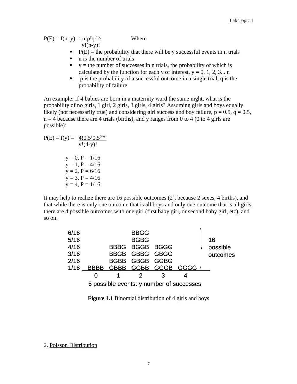y = 0, P = 1/16 y = 1, P = 4/16 y = 2, P = 6/16 y = 3, P = 4/16 y = 4, P = 1/16 It may help to realize there are 16 possible outcomes (24, because 2 sexes, 4 births), and that while there is only one outcome that is all boys and only one outcome that is all girls, there are 4 possible outcomes with one girl (first baby girl, or second baby girl, etc), and so on. Figure 1.1 Binomial distribution of 4 girls and boys 2. Poisson Distribution BBBB GGGG GBBB BGBB BBGB BBBG GGGB GGBG GBGG BGGG GGBB GBGB BGBG GBBG BGGB BBGG 0 1 2 3 4 1/16 2/16 3/16 4/16 5/16 6/16 5 possible events: y number of successes 16 possible outcomes BBBB GGGG GBBB BGBB BBGB BBBG GGGB GGBG GBGG BGGG GGBB GBGB BGBG GBBG BGGB BBGG 0 1 2 3 4 1/16 2/16 3/16 4/16 5/16 6/16 5 possible events: y number of successes 16 possible outcomes 7 Lab Topic 1 The Poisson distribution expresses the probability of the number of events in a given period of time or sample size, based on a known average frequency. When the average probability (p) of an event is rare (such as a specific mutation) in the sample size (such as a large region of DNA or many DNAs), the Poisson distribution becomes useful. The Poisson distributions can be derived from the Binomial distribution. P(E) = f(y,λ) = e - λ λ y y!  P(E) = the probability that there will be y successes  e = base of natural logarithm  y = the number of successes, the probability of which is calculated by the function for each y of interest, y = 0, 1, 2, 3... 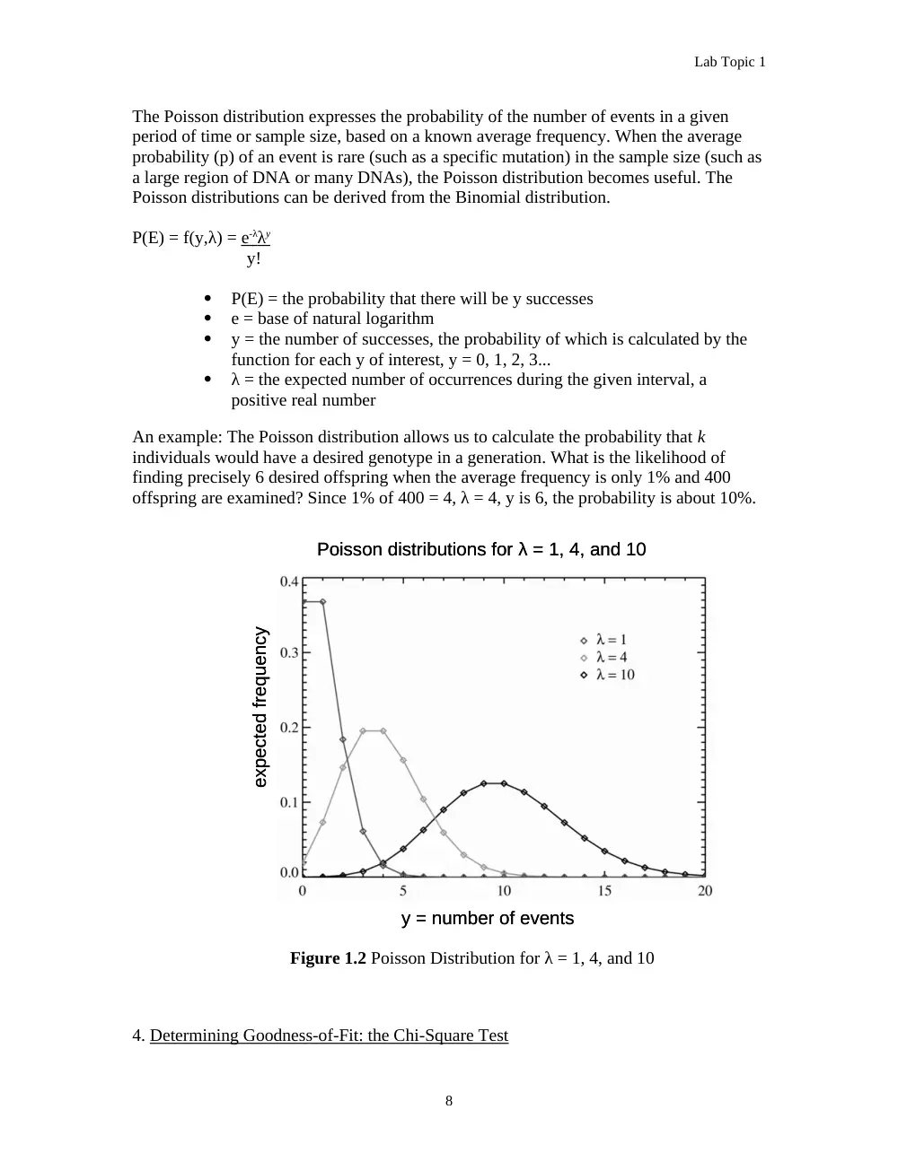 λ = the expected number of occurrences during the given interval, a positive real number An example: The Poisson distribution allows us to calculate the probability that k individuals would have a desired genotype in a generation. What is the likelihood of finding precisely 6 desired offspring when the average frequency is only 1% and 400 offspring are examined? Since 1% of 400 = 4, λ = 4, y is 6, the probability is about 10%. Figure 1.2 Poisson Distribution for λ = 1, 4, and 10 4. 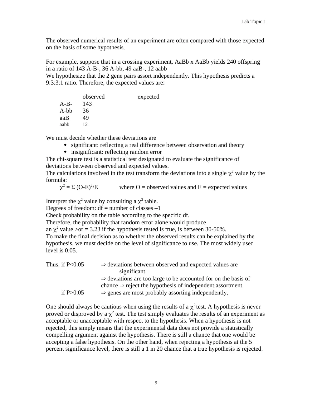Determining Goodness-of-Fit: the Chi-Square Test Poisson distributions for λ = 1, 4, and 10 y = number of events expected frequency Poisson distributions for λ = 1, 4, and 10 y = number of events expected frequency 8 Lab Topic 1 The observed numerical results of an experiment are often compared with those expected on the basis of some hypothesis. For example, suppose that in a crossing experiment, AaBb x AaBb yields 240 offspring in a ratio of 143 A-B-, 36 A-bb, 49 aaB-, 12 aabb We hypothesize that the 2 gene pairs assort independently. This hypothesis predicts a 9:3:3:1 ratio. Therefore, the expected values are: observed expected A-B- 143 A-bb 36 aaB 49 aabb 12 We must decide whether these deviations are  significant: reflecting a real difference between observation and theory  insignificant: reflecting random error The chi-square test is a statistical test designated to evaluate the significance of deviations between observed and expected values. The calculations involved in the test transform the deviations into a single 2 value by the formula: 2 = Σ (O-E)2/E where O = observed values and E = expected values Interpret the 2 value by consulting a 2 table. Degrees of freedom: df = number of classes –1 Check probability on the table according to the specific df. Therefore, the probability that random error alone would produce an 2 value >or = 3.23 if the hypothesis tested is true, is between 30-50%. To make the final decision as to whether the observed results can be explained by the hypothesis, we must decide on the level of significance to use. The most widely used level is 0.05. Thus, if P<0.05  deviations between observed and expected values are significant  deviations are too large to be accounted for on the basis of chance  reject the hypothesis of independent assortment. if P>0.05  genes are most probably assorting independently. One should always be cautious when using the results of a 2 test. A hypothesis is never proved or disproved by a 2 test. The test simply evaluates the results of an experiment as acceptable or unacceptable with respect to the hypothesis. When a hypothesis is not rejected, this simply means that the experimental data does not provide a statistically compelling argument against the hypothesis. There is still a chance that one would be accepting a false hypothesis. On the other hand, when rejecting a hypothesis at the 5 percent significance level, there is still a 1 in 20 chance that a true hypothesis is rejected. 9 Lab Topic 1 IV. Report Form Biology 223: Lab 1-Probability Name_____________________ Lab Partner_______________________________ Date______________________ Lab Section & Instructor____________________ 1. Shaved Dice Six-sided dice are commonly used to generate random numbers in games of chance. One method to cheat is to use biased dice to alter the frequency of specific numbers. There are many methods to bias dice. Here, you are given a pair of dice, one shaved, and one normal, and each numbered in binary code with short (0) and long (1) grooves. Note that the identification grooves may also bias the normal die. 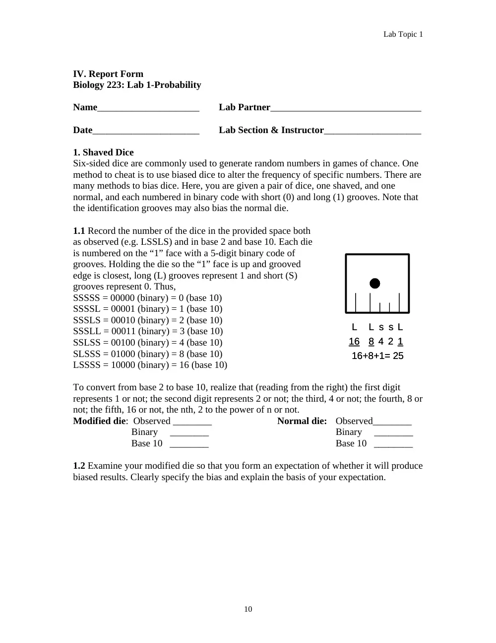1.1 Record the number of the dice in the provided space both as observed (e.g. LSSLS) and in base 2 and base 10. Each die is numbered on the “1” face with a 5-digit binary code of grooves. Holding the die so the “1” face is up and grooved edge is closest, long (L) grooves represent 1 and short (S) grooves represent 0. Thus, SSSSS = 00000 (binary) = 0 (base 10) SSSSL = 00001 (binary) = 1 (base 10) SSSLS = 00010 (binary) = 2 (base 10) SSSLL = 00011 (binary) = 3 (base 10) SSLSS = 00100 (binary) = 4 (base 10) SLSSS = 01000 (binary) = 8 (base 10) LSSSS = 10000 (binary) = 16 (base 10) To convert from base 2 to base 10, realize that (reading from the right) the first digit represents 1 or not; the second digit represents 2 or not; the third, 4 or not; the fourth, 8 or not; the fifth, 16 or not, the nth, 2 to the power of n or not. Modified die: Observed ________ Normal die: Observed________ Binary ________ Binary ________ Base 10 ________ Base 10 ________ 1.2 Examine your modified die so that you form an expectation of whether it will produce biased results. Clearly specify the bias and explain the basis of your expectation. 4 16 8 2 1 L L s L s 16+8+1= 25 4 16 8 2 1 L L s L s 16+8+1= 25 10 Lab Topic 1 1.3 State your expectation as a hypothesis, that you can indirectly test using Chi-square. What’s the name of this hypothesis? 1.4 State the complementary hypothesis. What is the name of this hypothesis? 1.5 Using a cup, and shaking with reasonable vigor, cast the dice. To make efficient use of time and to reduce errors, one partner should call the numbers; the other partner should record the results in the following table. Data should be recorded in non-erasable ink, errors should be indicated by a single slash through the error, and the corrected result should be entered next to the error. If a die does not land in the intended area, or does not land flat, disregard the roll. roll die # die# roll die# die# roll die# die# roll die# die# 1 25 49 73 2 26 50 3 27 4 28 5 29 6 30 7 8 80 9 10 11 12 60 13 14 15 16 40 17 18 90 19 20 21 22 70 23 11 Lab Topic 1 24 48 72 96 roll die # die# roll die# die# roll die# die# roll die# die# 97 121 145 169 170 100 150 130 180 110 160 140 190 120 144 168 192 12 Lab Topic 1 roll die # die# roll die# die# roll die# die# roll die# die# 193 200 204 1.6 After rolling the dice 204 times, summarize the number of times each face was up, Die # _____ Die # _____ 1.7 For the non-modified die, formulate a hypothesis that you can test using chi-square 1 2 3 4 5 6 1 2 3 4 5 6 13 Lab Topic 1 1.8 Apply a chi-squared test to your hypothesis. O E O-E (O-E)2 (O-E)2/E Total 2 1.9 Discuss your results. 1.10 Now test the hypothesis you made for the modified die O E O-E (O-E)2 (O-E)2/E Total 2 1.11 Discuss you results. Decide whether you should reconsider your hypothesis, or whether you have time to increase the confidence of your results by more rolls. 14 Lab Topic 1 2. Random Sampling You will be given a container with thoroughly mixed equal quantities of beads or beans of 2 different colors. Procedure: 2.1 Remove a random sample of the mixture 2.2 Separate and count the beads of different colors 2.3 Record your data: White: Colored: 2.4 What are your predictions with respect to the numbers of beads in the sample? Evaluate the deviations from the predicted values using 2analysis. O E O-E (O-E)2 (O-E)2/E Total 2 2.5 How many degrees of freedom do you have in the interpretation of the 2 value? 2.6 What is the probability that the observed deviations are only due to chance? 2.7 Interpret you results 3. Probability Distribution You will get a large mixture of beads of 2 different colors in exactly equal numbers. Assume that the beads represent the alleles for pigment production gene; the colored beads represent the allele for normal pigmentation and the white beads represent the alleles for albinism. 15 Lab Topic 1 Suppose that you marry a person who has a normal pigmentation just like you, but that both of you are carriers of the allele for albinism. The 2 alleles will be present in equal amounts in your gametes. Procedure: 3.1 Draw 2 beads from the jar to represent the genes in a sperm and an egg. 3.2 Write the genotype of your first child using appropriate gene symbols 3.3 Return the beads to the jar and draw 3 other pairs, one after the other 3.4 Record the genotypes and phenotypes of your 4 children? First Child Second Child Third Child Fourth Child Phenotype Genotype 3.5 What is the ratio of normal to albino phenotypes among your children? ________ Normal:________ Albino 3.6 What is the probability of getting the combination you obtained in a cross between 2 heterozygotes? 3.7 What is the chance of getting each of the 4 other combinations? 16 Lab Topic 1 3.8 Tabulate the results of the entire class All Normal 3 Normal: 1 Albino 2 Normal: 2 Albino 1 Normal: 3 Albino All Albinos 3.9 Is the hypothesis that the class data approximates the ratio expected from the binomial expansion accepted or not? Interpret your results. 17 Lab Topic 2 Lab Topic 2-Classical Mendelian Genetics in Drosophila Layane Hajjar I. Introduction Drosophila melanogaster, the common fruit fly, has been subject of extensive genetic studies since 1909 and is still important. Its success as a model organism is due to many characteristics: it has a short life cycle passing through complete metamorphosis in 10- 14 days at 20-25˚C, it produces large numbers of offspring (a single female can lay as many as 500 eggs in 10 days), it is inexpensive, and can be easily raised in the laboratory. It also shows great genetic variability. Many spontaneous mutations have been identified in Drosophila and many others have been introduced through radiation. Some of these mutations produce readily identifiable phenotypes. Also, many aspects of gene transmission and sex determination are similar to other animals, including humans. In this lab, you will use Drosophila melanogaster to perform monohybrid and diybrid genetic crosses and interpret F2 data that illustrate Mendel’s laws of segregation and independent assortment. II. Student Learning Outcomes In completing this activity, students should be able to: - Understand and explain why Drosophila melanogaster is a very useful model organism. - Prepare and passage fruit fly cultures. - Handle and examine fruit flies with anesthesia and microscopic examination. - Design experimental monohybrid and dihybrid crosses to verifiy Mendel’s first and second laws. - Accurately record the results of Drosophila breeding experiment. - Interpret F2 data illustrating Mendel’s first and second laws. - Statistically test for the goodness of fit of F2 data. III. Background A. Drosophila Life Cycle Drosophila melanogaster is a holometabolous insect (order Diptera, true flies) showing complete metamorphosis with four different stages: egg, larva, pupa and adult (Figure 2.1). Under optimal conditions, new adults can be produced in 2 weeks: 8 days in the egg and larval stages, and 6 days in the pupa stage. After their emergence from the puparium, the adults can live up to 8 weeks. They are ready for mating within 10 hours. The eggs are very small, about 0.5mm long, and are usually laid on the surface of the culture medium. One day after the eggs are laid, minute larvae hatch out and start feeding on yeast cells found in the medium. These first instar larvae double in size within 24 hours. In 2 days, they undergo a molt, and develop into second instar larvae that will similarly eat, grow and molt their cuticle to become third instar larvae that are about 5mm long and can be seen on the culture medium. The third instar larvae then crawl up out of the food and adhere to a relatively dry surface. Then the larval cuticle hardens and darkens to become the pupa case or puparium. During pupation, which lasts for about 6 days, metamorphosis from the larval to the adult form takes place. About one day before the emergence of the adult, the puparium darkens, the folded wings appear as dark elliptical 18 Lab Topic 2 bodies, and the eye pigment becomes visible through the puparium. The adult emerges by forcing its way through the anterior end of the pupa case. When it first emerges, it is light in color with folded wings and a long abdomen. In few hours, the wings expand, the body becomes more compact and the color gradually darkens. In about 10 hours, the adults would be ready for mating Figure 2.1 Drosophila melanogaster life cycle B. Distinguishing Sex in Drosophila In order to perform genetic crosses, it is essential to correctly identify the sex of the fruit flies. This should be done by a close examination of the