CIVE 440 Notes Instructor Notes, Fall 2012

Hydraulics & Laboratory September 2012 Printing History: Sep. 2005; Oct. 2006; Oct. 2009; Feb. 2010; Nov. 2011; Sep. 2012 Hydraulics & Laboratory Syllabus Syllabus Semester: Fall 2012 Course No: CIVE 440 Course Title: Hydraulics & Laboratory Prerequisites: CIVE 340 Fluid Mechanics Class Schedule: Tu. & Th. 12:30–13:50; Tu. & Th. 14:00–15:20 or On-Call-Basis Classroom: Bechtel Rm. 545 Instructor: Habib Basha Office: Bechtel Rm. 535 Hours: Tu. & Th.: 11:30–12:30 & 15:30–16:30 or by appointment Topics Flow in Conduits; Flow in Open-Channels; Flow Measurements; Laboratory Experiments. Textbook Crowe, C. T., Elger, D. F., and Roberson, J. A., Engineering Fluid Mechanics, 9th ed., chap. 10, 13, & 15, John Wiley & Sons, New York, 2010. Course Description Hydraulics deals with the application of fluid mechanics in the analysis and design of hydraulic structures and water resources systems. The course is important in that it provides the technical background in the design of water resources projects. The primary applications are in the analysis of flow in water distribution systems and the design of canals and related structures for irrigation projects. Another important application is in measurements of discharge in conduits and in channels. The course is divided in two main parts covering pipe flow and open-channel flow. Laboratory experiments dealing with flow measurements and pipe friction are also conducted. Course Learning Outcomes  Students will know the fundamental hydraulic concepts.  Students will have the ability to solve pipe-flow problems.  Students will have the ability to compute water-surface profiles in open-channels.  Students will have the ability to design basic hydraulic structures.  Students will have the ability to measure discharge in water systems.  Students will have had a hands-on experience of hydraulics in the laboratory.  Students will be skilled in the use of major technical software.  Students will have basic technical writing skills. 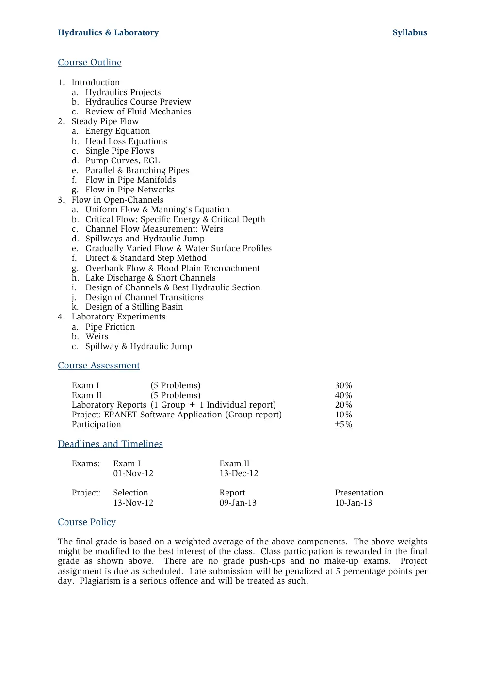Hydraulics & Laboratory Syllabus Course Outline 1. Introduction a. Hydraulics Projects b. Hydraulics Course Preview c. Review of Fluid Mechanics 2. Steady Pipe Flow a. Energy Equation b. Head Loss Equations c. Single Pipe Flows d. Pump Curves, EGL e. Parallel & Branching Pipes f. Flow in Pipe Manifolds g. Flow in Pipe Networks 3. Flow in Open-Channels a. Uniform Flow & Manning’s Equation b. Critical Flow: Specific Energy & Critical Depth c. Channel Flow Measurement: Weirs d. Spillways and Hydraulic Jump e. Gradually Varied Flow & Water Surface Profiles f. Direct & Standard Step Method g. Overbank Flow & Flood Plain Encroachment h. Lake Discharge & Short Channels i. Design of Channels & Best Hydraulic Section j. Design of Channel Transitions k. Design of a Stilling Basin 4. Laboratory Experiments a. Pipe Friction b. Weirs c. Spillway & Hydraulic Jump Course Assessment Exam I (5 Problems) 30% Exam II (5 Problems) 40% Laboratory Reports (1 Group + 1 Individual report) 20% Project: EPANET Software Application (Group report) 10% Participation 5% Deadlines and Timelines Exams: Exam I Exam II 01-Nov-12 13-Dec-12 Project: Selection Report Presentation 13-Nov-12 09-Jan-13 10-Jan-13 Course Policy The final grade is based on a weighted average of the above components. The above weights might be modified to the best interest of the class. Class participation is rewarded in the final grade as shown above. There are no grade push-ups and no make-up exams. Project assignment is due as scheduled. Late submission will be penalized at 5 percentage points per day. Plagiarism is a serious offence and will be treated as such. 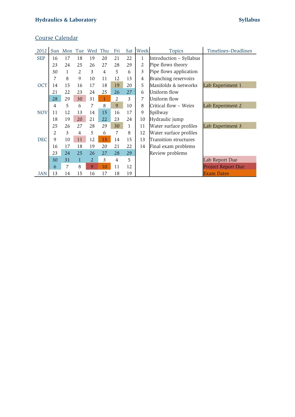Hydraulics & Laboratory Syllabus Course Calendar 2012 Sun Mon Tue Wed Thu Fri Sat Week Topics Timelines–Deadlines SEP 16 17 18 19 20 21 22 1 Introduction – Syllabus 23 24 25 26 27 28 29 2 Pipe flows theory 30 1 2 3 4 5 6 3 Pipe flows application 7 8 9 10 11 12 13 4 Branching reservoirs OCT 14 15 16 17 18 19 20 5 Manifolds & networks Lab Experiment 1 21 22 23 24 25 26 27 6 Uniform flow 28 29 30 31 1 2 3 7 Uniform flow 4 5 6 7 8 9 10 8 Critical flow – Weirs Lab Experiment 2 NOV 11 12 13 14 15 16 17 9 Spillway 18 19 20 21 22 23 24 10 Hydraulic jump 25 26 27 28 29 30 1 11 Water surface profiles Lab Experiment 3 2 3 4 5 6 7 8 12 Water surface profiles DEC 9 10 11 12 13 14 15 13 Transition structures 16 17 18 19 20 21 22 14 Final exam problems 23 24 25 26 27 28 29 Review problems 30 31 1 2 3 4 5 Lab Report Due 6 7 8 9 10 11 12 Project Report Due JAN 13 14 15 16 17 18 19 Exam Dates Hydraulics & Laboratory Table of Contents Table of Contents Hydraulics & Laboratory ..................................................................................................... i Syllabus ............................................................................................................................ iii Table of Contents ............................................................................................................. vii 1. Introduction .................................................................................................................. 1 1.1 Water Networks ....................................................................................................... 1 1.2 Irrigation System ...................................................................................................... 2 2. Steady Pipe Flows ......................................................................................................... 3 2.1 Continuity Equation ................................................................................................. 3 2.2 Energy Equation ....................................................................................................... 3 2.3 Laminar and Turbulent Flow .................................................................................... 4 2.4 Head Loss Equations ................................................................................................ 4 2.4.1 Pipe Friction Losses ........................................................................................ 4 2.4.2 Pipe Fitting Losses .......................................................................................... 5 2.5 Power, EGL and HGL ............................................................................................... 5 2.6 Solution of Pipe-Flow Problems ................................................................................ 5 2.7 Conduit Systems .................................................................................................... 11 3. Flow in Open-Channels ................................................................................................ 21 3.1 Uniform Flow ......................................................................................................... 21 3.1.1 Manning’s Equation ...................................................................................... 21 3.1.2 Compound Channel ...................................................................................... 22 3.1.3 Best Hydraulic Section................................................................................... 22 3.1.4 Flood Plain Encroachment ............................................................................. 22 3.1.5 Design of Erodible Channels .......................................................................... 22 3.2 Critical Flow .......................................................................................................... 22 3.3 Energy Equation ..................................................................................................... 23 3.4 Weirs..................................................................................................................... 24 3.4.1 Broad-crested weirs ....................................................................................... 24 3.4.2 Sharp-crested weirs ....................................................................................... 24 3.5 Hydraulic Jump ...................................................................................................... 25 3.6 Gradually Varied Flow ............................................................................................ 25 3.6.1 Direct Step Method ....................................................................................... 26 3.6.2 Standard Step Method ................................................................................... 26 3.7 Flood Plain Delineation .......................................................................................... 26 3.8 Design of Channel Transitions ................................................................................ 27 Appendix ......................................................................................................................... 39 Homework Problems 2006 .............................................................................................. 107 Homework Problems 2008 .............................................................................................. 118 Homework Problems 2009 .............................................................................................. 129 Homework Problems 2010S ............................................................................................. 140 Homework Problems 2010F ............................................................................................. 146 Homework Problems 2011 .............................................................................................. 152 Homework Problems 2011F ............................................................................................. 158 Experiments ................................................................................................................... 165 Formulae Sheet I ................................................................................................................ 1 Formulae Sheet II ............................................................................................................... 2 1 1. Introduction Hydraulic engineering deals with the analysis and design of hydraulic structures and water resources systems. The primary applications are in the analysis of flow in water distribution systems and the design of canals and related structures for irrigation projects. Another important application is in measurements of discharge in conduits and in channels. 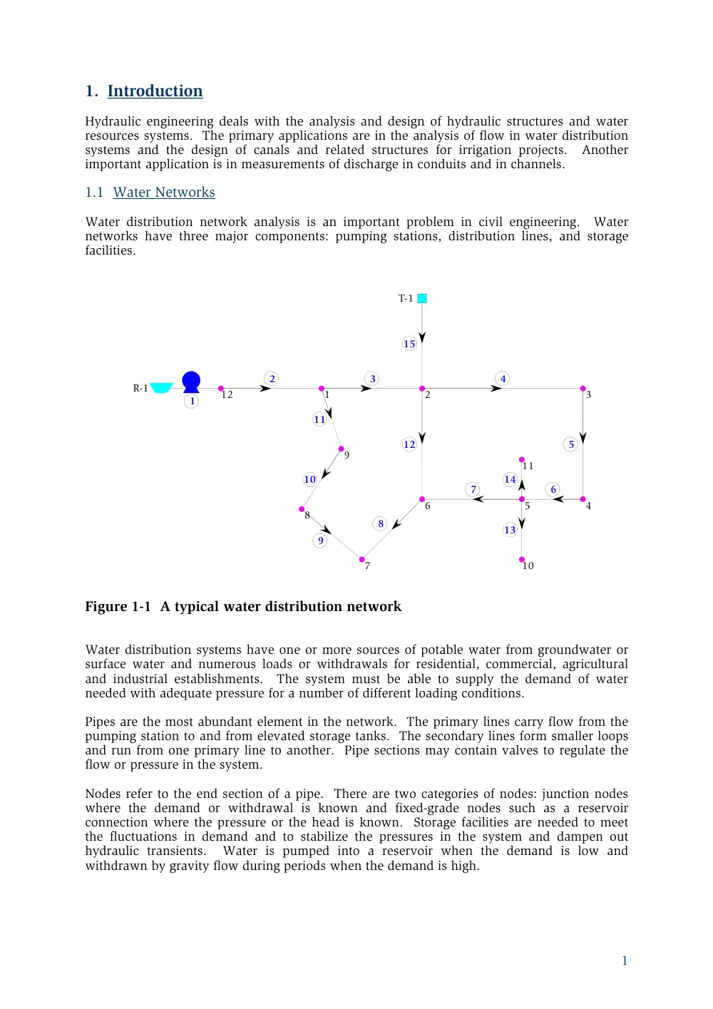1.1 Water Networks Water distribution network analysis is an important problem in civil engineering. Water networks have three major components: pumping stations, distribution lines, and storage facilities. 1 2 3 4 5 6 7 8 9 10 11 12 13 14 15 1 2 3 4 5 6 7 8 9 10 11 12 R-1 T-1 Figure 1-1 A typical water distribution network Water distribution systems have one or more sources of potable water from groundwater or surface water and numerous loads or withdrawals for residential, commercial, agricultural and industrial establishments. The system must be able to supply the demand of water needed with adequate pressure for a number of different loading conditions. Pipes are the most abundant element in the network. The primary lines carry flow from the pumping station to and from elevated storage tanks. The secondary lines form smaller loops and run from one primary line to another. Pipe sections may contain valves to regulate the flow or pressure in the system. Nodes refer to the end section of a pipe. There are two categories of nodes: junction nodes where the demand or withdrawal is known and fixed-grade nodes such as a reservoir connection where the pressure or the head is known. Storage facilities are needed to meet the fluctuations in demand and to stabilize the pressures in the system and dampen out hydraulic transients. Water is pumped into a reservoir when the demand is low and withdrawn by gravity flow during periods when the demand is high. 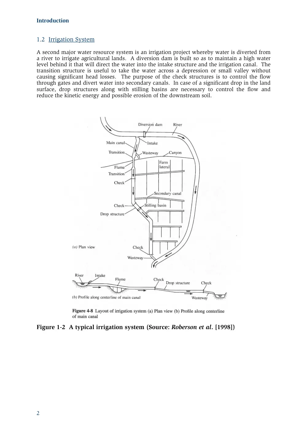Introduction 2 1.2 Irrigation System A second major water resource system is an irrigation project whereby water is diverted from a river to irrigate agricultural lands. A diversion dam is built so as to maintain a high water level behind it that will direct the water into the intake structure and the irrigation canal. The transition structure is useful to take the water across a depression or small valley without causing significant head losses. The purpose of the check structures is to control the flow through gates and divert water into secondary canals. In case of a significant drop in the land surface, drop structures along with stilling basins are necessary to control the flow and reduce the kinetic energy and possible erosion of the downstream soil. Figure 1-2 A typical irrigation system (Source: Roberson et al. [1998]) 3 2. Steady Pipe Flows Flow in conduits arises in many fields of engineering. Water distribution systems are one prime application of the theory of conduit flows. The basic principles governing closed conduit flows are: conservation of mass, conservation of energy, and conservation of momentum. The continuity and energy equations are used to design a pipe system, while the momentum equation is employed to determine the forces acting on bends for a given discharge. 2.1 Continuity Equation The continuity equation is expressed by dS Q Q dt   in out (2.1) where in Q and Qout are the flow rates entering and exiting the system, and S is the volume of water stored in the system. For steady flow, eq. (2.1) simplifies to in out Q  Q or A V A V  in in out out (2.2) where A is the cross-sectional area of the flow. 2.2 Energy Equation The energy equation is given by p t L p V p V z h z h h g g             2 2 1 1 2 2 1 1 2 2 2 2 (2.3) where p  is the pressure head (i.e. the energy possessed by the liquid in virtue of its pressure), V2 2 g is the velocity head (i.e. the kinetic energy per unit weight of a flowing liquid), z is the elevation head (potential energy), p h is the head supplied by the pump, th is the head supplied by the turbine, and L h is the head loss between section 1 and 2. The correction factor  in the velocity head term accounts for the assumption of a mean velocity in (2.3) whereas the actual velocity distribution is varying from a maximum at the centerline to zero at the boundaries u dA   AV  3 3 1 (2.4) Here u is the actual velocity distribution and V is the mean velocity. The parameter  ranges from 1.01 to 1.15 and is usually assumed to be unity in pipe flow computations. The sum of the pressure head, the velocity head, and the elevation head is defined as the hydraulic head H p V H z g     2 2 (2.5) Water flows from a higher head H to a lower head. Eq. (2.3) can then be expressed as 1 2 p t L H h H h h     . It applies to incompressible steady flow of a real viscous fluid flowing from an inlet section to an outlet section. If L h  0 , the fluid is assumed to be inviscid, i.e. frictionless. For p t L h h h    0 , eq. (2.3) reduces to the Bernoulli equation. Steady Pipe Flows 4 2.3 Laminar and Turbulent Flow Flow of water is mostly turbulent; the flow of oil can be laminar. The flow is considered laminar when the Reynolds number is less than 2000, and it is turbulent for Reynolds number greater than 3000. The velocity profile in laminar flows is parabolic while the velocity distribution in turbulent flows is of the form of a power law formula. 2.4 Head Loss Equations 2.4.1 Pipe Friction Losses In laminar flows, the head loss is proportional to V. The mathematical equations become easier to solve since they are linear. On the other hand, the head loss in turbulent flows is proportional to n V . The governing equations are therefore nonlinear and more difficult to solve. Dimensional analysis and experimental investigations are used to come up with the head loss equation. For laminar flow in pipes, the friction equation can be derived from the shear stress distribution and the parabolic velocity distribution. It is expressed by f LV h D    2 32 (2.6) For turbulent flows, the head loss in a pipe is given by L L V h f D g  2 2 (2.7) The friction factor f can be found from the Moody diagram or from the following equation valid for sk D     5 2 10 2.10 and for  R  8 e 4000 10 s e k D f R f            1 2.51 2log 3.7 (2.8) An alternate equation, which expresses the friction factor f in an explicit fashion, is given by s e f k D R               2 10 0.9 0.25 5.74 log 3.7 (2.9) For noncircular pipes, the friction equation (2.7) becomes L h f L V h R g  2 4 2 (2.10) where the hydraulic radius h R is defined as h A R  P (2.11) Here A is the cross-sectional area of the flow and P is the wetted perimeter. For a circular pipe flowing full, Rh  D 4 . The hydraulic radius concept is substituted for D in non- circular cross sections and is used extensively in open channel flows and free surface flows. Power, EGL and HGL 5 2.4.2 Pipe Fitting Losses Besides the friction loss in the pipe, there are also minor losses in pipe fittings, bends, valves, entrances and exits. All minor losses are expressed in terms of m V h k g  2 2 (2.12) where k is the loss coefficient (for entrance losses, sudden contraction and expansion, pipe fittings) given in figures and tables in textbooks. For submerged exit loss, k  1. 2.5 Power, EGL and HGL The power in Watts is expressed as P  QH (2.13) where H is the head. The power of a jet is for H V g  2 2 , the power lost in fluid friction is for L H  h , and the power of a machine is for m H  h . The hydraulic grade line (HGL) is the sum of the pressure and elevation head p   z , and the energy grade line (EGL) is the plot of the hydraulic head H (2.5). The EGL decreases at a rate of head loss. The HGL and EGL are useful for spotting regions of low pressures without the need for calculating the pressure at fine discrete intervals. If the hydraulic grade line between two points fall below the pipe system, then that region has a low pressure. 2.6 Solution of Pipe-Flow Problems There are basically three types of problems: 1. Determine the head loss, given the flow rate, kind and size of pipe. 2. Determine the flow rate, given the head, kind and size of pipe 3. Determine the size of pipe, given the head, flow rate, and kind of pipe. The solution of pipe flow problems consists of writing the energy equation between any two points for which the pressure and/or velocity are known. If there are two unknowns, one must use the continuity equation also. The solution of some problems might involve a trial and error procedure to find the velocity or flow rate. Remember that all relevant loss terms must be included. Steady Pipe Flows 6 Example 2.1: Minimum Pressure Calculate the discharge in the pipe and determine the points of maximum and minimum pressure in the system. Assume Kb  0.2,   1.22 x10 -5 ft 2/s and   62.4 lb/ft 3. Solution Expressing the energy equation between point 1 at the reservoir and point 2 at the free jet, one obtains t m P V P V L V z h z f k g g D g                   2 2 2 1 1 2 2 2 1 2 2 2 2 Therefore, V f g            12 100 100 64 1 0.5 0.2 1 2 Assuming f  0.028, one obtains V  22.7 ft/s and Re  1.9 x 10 6 and the new value of f is f  0.028. No further iteration is needed. The flow rate is then Q  17.58 ft/s. The point of minimum pressure is at the entrance of the pipe or at the exit, i.e. zero. The pressure at the entrance is     eP g      22.7 2 100 95 1 0.5 2 Hence. Pe  7, i.e. Pe  3 psig is the minimum pressure. The maximum pressure is just before the bend   Pm g             22.7 2 72 100 44 1 0.5 0.028 1 2 Hence, Pm  27.9 (62.4)  1740 lb/ft 2 is the maximum pressure. Solution of Pipe-Flow Problems 7 Example 2.2: Loss Coefficient Compute the loss coefficient Kv of the partially-closed valve that reduces the discharge to 50% of the flow with the valve wide open. The equivalent sand-grain roughness of steel ks is 0.046 mm and the kinematic viscosity is 1.31 x 10 -6 m 2/s Solution Expressing the energy equation between the two reservoirs, one obtain   V f g            2 14 2 0.5 2 0.9 .2 1 0.1 2 Assuming f  0.018, one gets V  2.55 m/s. Iterating again, one obtains f  0.0188 and the velocity becomes V  2.53 m/s. The flow rate is then Q  0.02 m 3/s. For one-half the discharge, Q  0.01 m/s, the corresponding velocity is V  1.27 m/s. The corresponding f  0.02. Hence   vk g            2 14 1.27 2 0.5 2 0.9 1 .02 0.1 2 Solving for Kv, one gets Kv  18.2. Steady Pipe Flows 8 Example 2.3: Turbine Problem Water drains from a pressurized tank through a pipe system as shown in the Figure. Compute the flow rate if the head of the turbine is equal to 116 m. The length of the pipe is 200 m. The fluid properties are   9.8 kN/m 3 and     1.12 10 6 m 2/s. Solution Expressing the energy equation between point 1 inside the tank and point 2 at the free jet, one obtains t m P V P V L V z h z f k g g D g                   2 2 2 1 1 2 2 2 1 2 2 2 2 Therefore, V f g              12 50 200 200 116 1 0.5 5 2 9.81 0.1 2 Here   V V Q    2 1 2 4 0.1 . Assuming f  0.03 , one obtains V  5.05 m/s. The Reynolds number is then e  5 R 4.5x10 and the new value of f is f  0.0354 . Further iteration yields V  4.69m/s and f  0.0355. The flow rate is then Q  VA  0.0368m 3/s. Solution of Pipe-Flow Problems 9 Example 2.4: Pump Curve Calculate the discharge of water in the following system Solution Expressing the energy equation between the lower reservoir and the upper reservoir, one obtains p V h g                12 1000 0 0 10 0 0 20 0.1 0.020 1 10 12 2 Now V Q A Q   1 0.545. Plotting this equation on the pump curve yields Q  2950gpm. Steady Pipe Flows 10 Example 2.5: Pipe Sizing Determine the pipe diameter needed for water (    6 1.14 x10 m 2/s) to flow from reservoir A to reservoir B through a cast-iron pipe (ks0.25 mm) of length 20 m at a rate of Q  0.002 m 3/s. The system contains a sharp-edged entrance (K0.5) and six threaded 90 o elbows (K1.5). Solution Expressing the energy equation between reservoir A and reservoir B, one obtains   V f D g                2 20 0 0 2 0 0 0 0.5 6 1.5 1 2 The solution proceeds by trial and error. One assumes D, solves for V using the continuity equation and determines f from the Moody’s diagram or s e f k D               2 0.9 0.25 5.74 log 3.7 R The results for various trial runs are tabulated below D A V Re f EB (cm) (m 2) (m/s) (m) 2 3.14 6.37 111690 0.0416 101.5 5 0.002 1.0186 44675 0.0327 1.089 4.5 0.0016 1.2575 49639 0.0334 1.802 4.4 0.0015 1.3153 50767 0.0336 2.007 Conduit Systems 11 2.7 Conduit Systems Flow in a series of pipes is the simplest pipe system. Other applications include flow in parallel pipes, flow in branching pipes, flow in a pipe manifold, and flow in pipe networks. For flow in pipes in parallel, the head loss is the same. The problem is to determine the division of flow in each pipe, given the total flow rate. Similarly, the problem of branching pipes is to determine the discharge in each pipe that is connected to a reservoir with a given head. Manifolds are pipes that branch into other pipes. They can be of the combining flow type or the dividing flow type. An example of a dividing flow type is a diffuser for disposal of sewage. The distribution of the flow can also be accomplished by ports cut in the manifold. The discharge through each port is different as the head in the pipe changes along the length of the manifold because of friction and momentum change. Problem 2.1: Parallel Pipes The pipes shown in the system are all concrete. Compute the head loss from A to B and the flow rates in the pipe system given that the total flow rate is 25 cfs. Steady Pipe Flows 12 Example 2.6: Branching Pipes Compute the flow rates and the elevation of the third reservoir given that the pipes are galvanized iron with sk  0.0005ft and     5 1.06 10 ft 2/s. N.B.: the flow rate value shown in pipe 1 is incorrect. Solution The piezometric head at point J is 112 ft. Expressing the energy equation between reservoir 1 and point J, one obtains for f  0.020 V g          12 1400 120 112 1 0.020 0.5 2 Hence V  1 3 ft/s and Q  1 0.6 cfs. Expressing the energy equation between reservoir 2 and point J, one obtains for f  0.020 V g          22 1800 124 112 1 0.020 8 12 2 Hence V  2 3.7 ft/s and Q  1 1.3cfs. From continuity, the flow rate in pipe 3 is 1.9 cfs and the velocity is then 3.5 ft/s. Expressing the energy equation between point J and reservoir 3, one obtains for f  0.020   z g           2 3 3.5 2400 112 1 0.020 101.2 10 12 2 ft The above values can be further corrected by updating the values of the friction coefficient using the Moody’s diagram: f  2 0.019 and f  3 0.018 . Conduit Systems 13 Example 2.7: Pipe Manifold System Compute the flow rates in a pipe manifold system and determine the water surface elevation in the upstream reservoir if the discharge rate at the last port in the dead end pipe is 2 cfs. The diameter of the manifold pipe is 12" and the diameter of the ports is 4". There are 5 discharge openings that are 10' spaced apart. The manifold is discharging into a pond at a depth of 10' and the distance from the reservoir to the first opening is 500'. Assume orifice flow in the ports with CD  0.675 and use a constant f  0.02. Solution The head at each port is obtained from the energy equation i i i i i i L V H H f D g    2 1 2 where s e k f D R                  2 10 0.9 1 5.74 4 log 3.7 The flow discharge through each port is given by   i i i i q K a g H H   0 2 where the flow coefficient K is   i i i V K g H H     2 1 0 0.675 1 2 The flow rates in the manifold system is obtained from the continuity equation at each port i i i Q Q q   1  The solution in tabular form is as follows: Port or q Q V K Re f hl H Segment (cfs) (cfs) (fps) 10 3 (ft) (ft) 5 2 0.6750 27.9008 4 1.9955 2 2.5465 0.6731 181.9 0.02 0.0201 27.9209 3 1.9831 3.9955 5.0872 0.6674 363.4 0.02 0.0804 28.0013 2 1.9651 5.9786 7.6122 0.6581 543.7 0.02 0.1800 28.1812 1 1.9439 7.9437 10.1142 0.6454 722.4 0.02 0.3177 28.4989 Rsv 9.8876 12.5893 899.2 0.02 24.6102 53.1091 Therefore, the water surface elevation in the reservoir should be 53 ft. Steady Pipe Flows 14 Example 2.8: Network – 8 Pipes Write down the system of equations for the given network and tabular data expressing all coefficients in numerical form. Determine also the head supplied by the pump. 1 2 3 4 5 6 7 1 2 3 4 5 6 7 8 The hydraulic data are: Junction 1 2 3 4 5 6 7 Elevation (m) 250 260 265 265 270 280 220 Demand (l/min) 0 0 150 50 0 100 RSV Pipe 1 2 3 4 5 6 7 8 Diameter (cm) 20 20 20 15 15 15 20 15 Length (m) 250 300 600 450 500 300 500 600 The pump curve is defined by the shutoff head of 200 m and the following curve points: (300 l/min, 180 m) and (600 l/min, 150 m). Use f  0.02 for all pipes. Solution There are 9 unknown pipe flow rates. The system of equation is then made of 6 continuity equations at the junctions and 3 energy equations around the 3 loops. The continuity equations are J-1: Qp Q Q    1 8 0 J-2: Q Q Q    1 7 2 0 J-3: Q Q Q    2 5 3 0.15 J-4: Q  Q  3 4 0.05 J-5: Q Q Q    6 5 4 0 J-6: Q Q Q    8 7 6 0.1 Loop 126: x x x k Q k Q k Q    1 1 7 7 8 8 0 Loop 2356: x x x x k Q k Q k Q k Q     2 2 5 5 6 6 7 7 0 Loop 345: x x x k Q k Q k Q    3 3 4 4 5 5 0 where fL k g D  2 5 8 Pipe 1 2 3 4 5 6 7 8 k (min 2/m 5) 0.3586 0.4303 0.861 2.720 3.023 1.814 0.7172 3.627 k (s 2/m 5) 1291 1549 3099 9793 10881 6529 2582 13057 The pump must supply a flow of 300 l/min; hence, the head supplied is 180 m. 21 3. Flow in Open-Channels The study of open-channel flows is essential to the computation of water surface profiles to define the levels of flood inundation. It is also important to the design of canals and related structures for irrigation projects. Open-channel flows are classified as uniform and non-uniform flows. Uniform flows assume that the velocity along the streamline is constant, i.e. 0 v x    . Hence, the depth is uniform across the length of the channel. This situation may occur in channels of constant cross- section and slope (prismatic channels). In case of uniform flow, the flow depth is called the normal depth and is designated by n y . The normal depth can be calculated using the Chezy equation or the more common Manning’s equation. Non-uniform flows are much more common than uniform flows. They are also two types of flow regimes in non-uniform flows: sub-critical flow (tranquil flow) and super-critical flow (rapid flow). In non-uniform flows, the flow is further classified into two categories based on the length over which the velocity and depth changes. For changes in y and V over short distances, the flow is classified as rapidly-varied flow, while for changes in y and V over a long stretch of the channel, the flow is referred to as gradually-varied flow. In rapidly-varied flow, the bottom friction is usually neglected because of the short distance, while in gradually-varied flows the friction is a significant component of the energy equation. Note that all the above flow classifications correspond to steady flows, i.e. 0 v t    . Unsteady uniform channel flow is beyond the scope of this chapter while the unsteady non-uniform flow is the most complicated open-channel flow and is reserved for advanced courses. The primary engineering application of flow in open-channels is the calculation of the flow depth y along the channel or river. In uniform flows, the depth is constant and is calculated once. In non-uniform flows, the depth is varyi