EECE 210 Homework 11 with Solution, Fall 2014

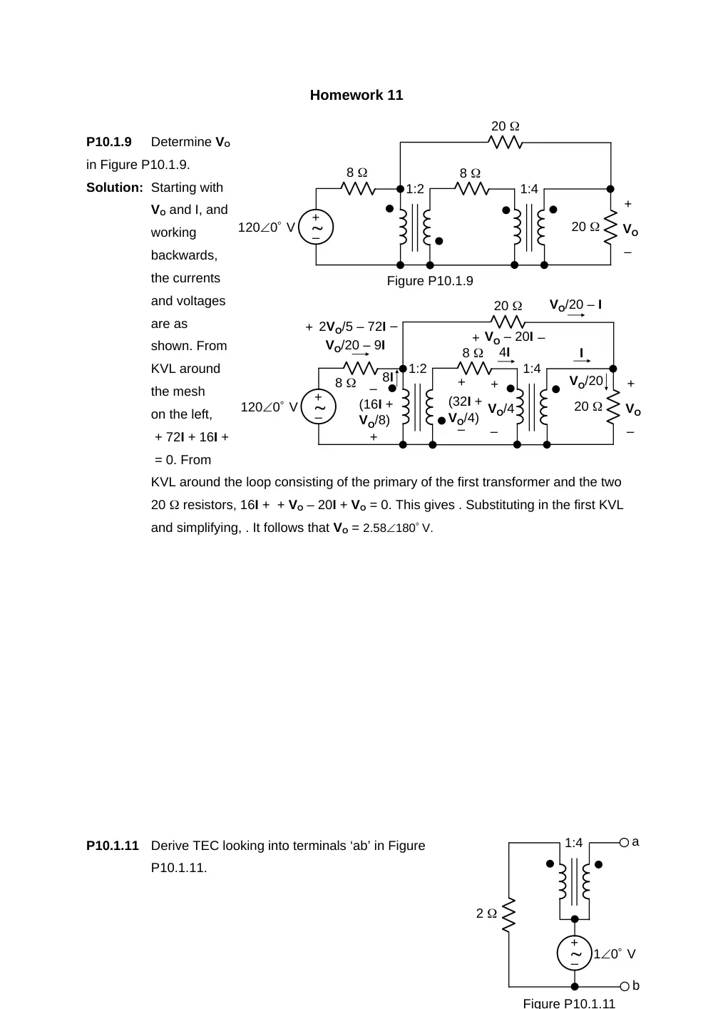
1:2 1200 V 8  1:4 – + 20  8  20  + – VO I VO/20 VO/20 – I + – VO – 20I 4I + – (32I + VO/4 VO/4) + – 8I (16I + VO/8) + – VO/20 – 9I + 2VO/5 – 72I – Homework 11 P10.1.9 Determine VO in Figure P10.1.9. Solution: Starting with VO and I, and working backwards, the currents and voltages are as shown. From KVL around the mesh on the left, + 72I + 16I + = 0. From KVL around the loop consisting of the primary of the first transformer and the two 20  resistors, 16I + + VO – 20I + VO = 0. This gives . Substituting in the first KVL and simplifying, . It follows that VO = 2.58180 V. P10.1.11 Derive TEC looking into terminals ‘ab’ in Figure P10.1.11. 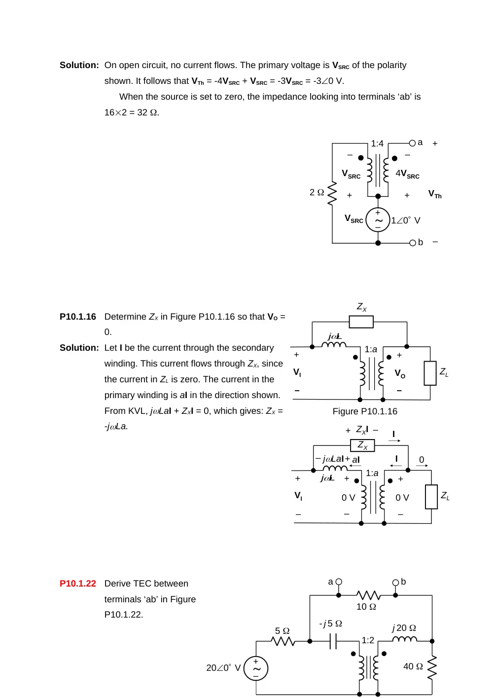1:2 1200 V Figure P10.1.9 8  1:4 – + 20  8  20  + – VO 1:4 2  Figure P10.1.11 10 V a b – + Solution: On open circuit, no current flows. The primary voltage is VSRC of the polarity shown. It follows that VTh = -4VSRC + VSRC = -3VSRC = -30 V. When the source is set to zero, the impedance looking into terminals ‘ab’ is 162 = 32 . P10.1.16 Determine ZX in Figure P10.1.16 so that VO = 0. Solution: Let I be the current through the secondary winding. This current flows through ZX, since the current in ZL is zero. The current in the primary winding is aI in the direction shown. From KVL, jLaI + ZXI = 0, which gives: ZX = -jLa. P10.1.22 Derive TEC between terminals ‘ab’ in Figure P10.1.22. 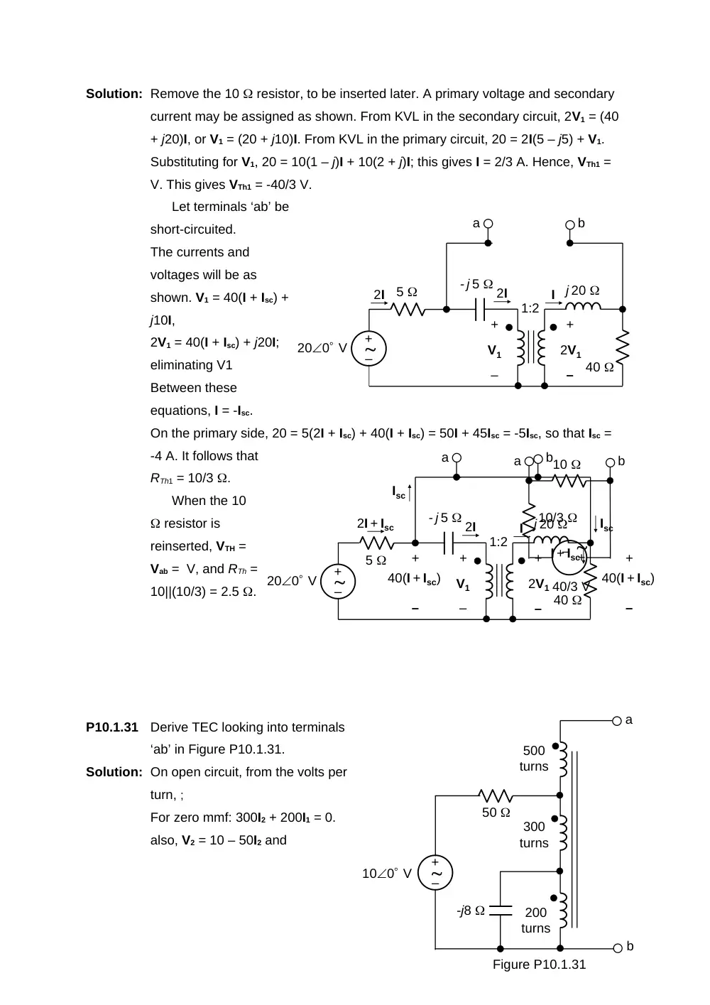1:4 2  10 V a b – + VSRC + – 4VSRC + – VSRC + – VTh + – VO ZL + – VI ZX L j 1:a Figure P10.1.16 + – 0 V + – VI ZX L j 1:a + – 0 V I aI I + jLaI ZL 0 – + – ZXI 200 V 5  - j 5  1:2 j 20  40  10  b a – + 200 V 5  - j 5  1:2 j 20  40  b a – + + – V1 + – 2V1 I 2I 2I + Isc Isc I + Isc 40(I + Isc) + – 40(I + Isc) + – Isc Solution: Remove the 10  resistor, to be inserted later. A primary voltage and secondary current may be assigned as shown. From KVL in the secondary circuit, 2V1 = (40 + j20)I, or V1 = (20 + j10)I. From KVL in the primary circuit, 20 = 2I(5 – j5) + V1. Substituting for V1, 20 = 10(1 – j)I + 10(2 + j)I; this gives I = 2/3 A. Hence, VTh1 = V. This gives VTh1 = -40/3 V. Let terminals ‘ab’ be short-circuited. The currents and voltages will be as shown. V1 = 40(I + Isc) + j10I, 2V1 = 40(I + Isc) + j20I; eliminating V1 Between these equations, I = -Isc. On the primary side, 20 = 5(2I + Isc) + 40(I + Isc) = 50I + 45Isc = -5Isc, so that Isc = -4 A. It follows that RTh1 = 10/3 . When the 10  resistor is reinserted, VTH = Vab = V, and RTh = 10||(10/3) = 2.5 . P10.1.31 Derive TEC looking into terminals ‘ab’ in Figure P10.1.31. Solution: On open circuit, from the volts per turn, ; For zero mmf: 300I2 + 200I1 = 0. 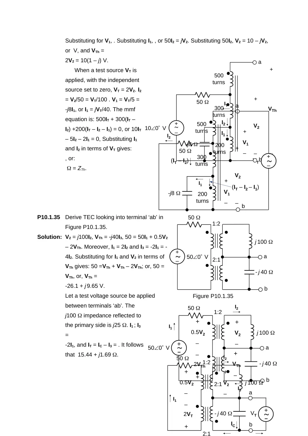also, V2 = 10 – 50I2 and 200 V 5  - j 5  1:2 j 20  40  b a – + + – V1 + – 2V1 I 2I 2I b a – +  40/3 V 10/3  10  500 turns 300 turns Figure P10.1.31 100 V 200 turns -j8  a b 50  – + Substituting for V1, . Substituting I1, , or 50I2 = jV2. Substituting 50I2, V2 = 10 – jV2, or V, and VTh = 2V2 = 10(1 – j) V. When a test source VT is applied, with the independent source set to zero, VT = 2V2. I2 = V2/50 = VT/100 . V1 = VT/5 = -j8I1, or I1 = jVT/40. The mmf equation is: 500IT + 300(IT – I2) +200(IT – I2 – I1) = 0, or 10IT – 5I2 – 2I1 = 0, Substituting I1 and I2 in terms of VT gives: , or:  = ZTh. P10.1.35 Derive TEC looking into terminal ‘ab’ in Figure P10.1.35. Solution: V2 = j100I2, VTh = j40I3, 50 = 50I1 + 0.5V2 – 2VTh. Moreover, I1 = 2I2 and I3 = -2I1 = - 4I2. Substituting for I1 and V2 in terms of VTh gives: 50 =VTh + VTh – 2VTh; or, 50 = VTh, or, VTh = -26.1 + j 9.65 V. Let a test voltage source be applied between terminals ‘ab’. The j100  impedance reflected to the primary side is j25 . I1 ; I3 = -2I1, and IT = IC – I3 = . It follows that 15.44 + j1.69 . 500 turns 300 turns 200 turns -j8  a b 50  – + IT I2 I1 + – V2 + – V1 (IT – I2) (IT – I2 – I1) VT 500 V 50  j 100  - j 40  1:2 2:1 a b Figure P10.1.35 – + – + 500 V 50  j 100  - j 40  1:2 2:1 a b + – 0.5V2 + – V2 + – VTh + – 2VTh I2 I1 I3  50  j 100  - j 40  1:2 2:1 a b + – 0.5V2 + – V2 + – 2VT I2 – + VT I1 IC 500 turns 300 turns 100 V 200 turns -j8  a b 50  – + + – V2 + – VTh + – V1 I1 I2 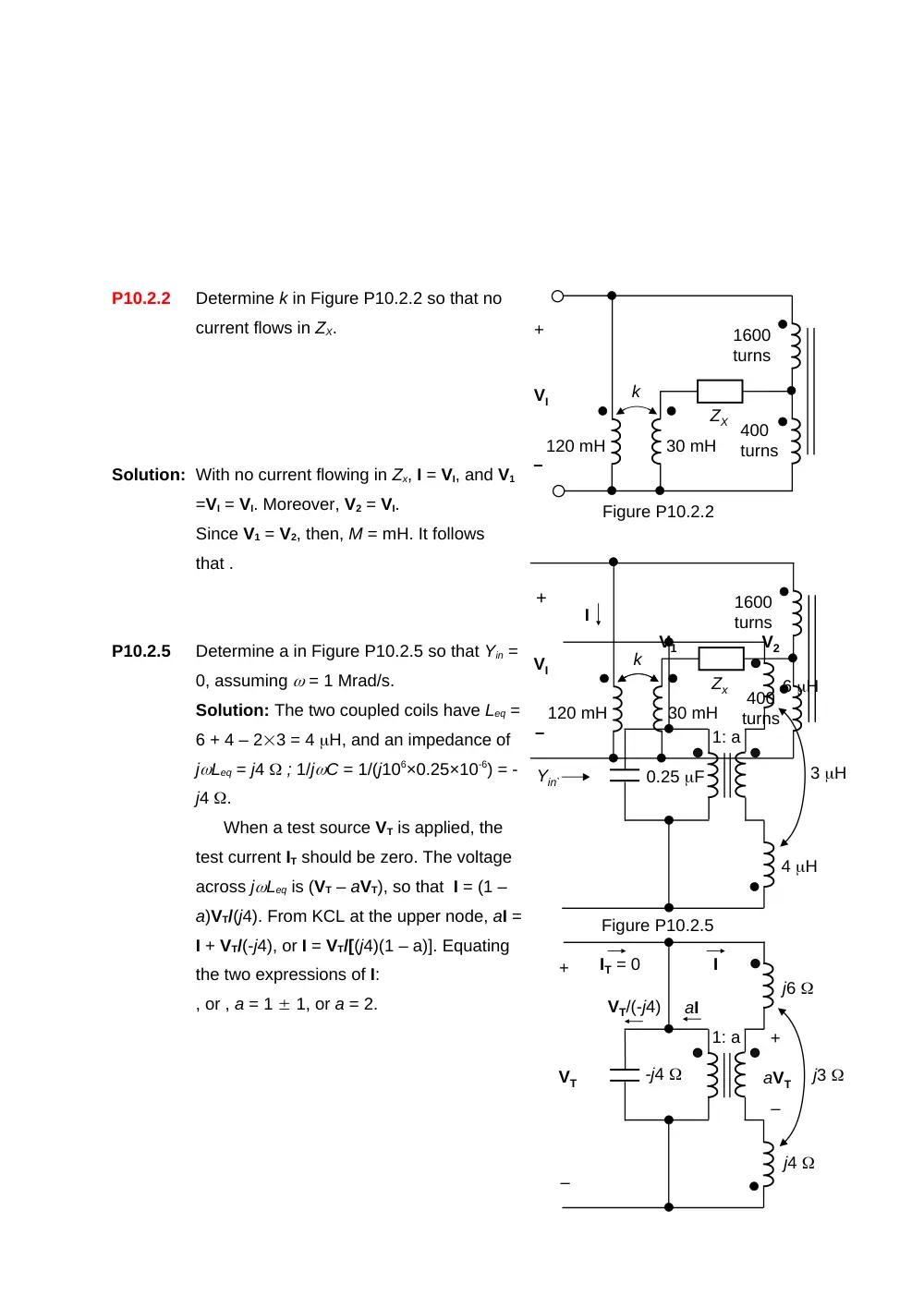P10.2.2 Determine k in Figure P10.2.2 so that no current flows in ZX. Solution: With no current flowing in Zx, I = VI, and V1 =VI = VI. Moreover, V2 = VI. Since V1 = V2, then, M = mH. It follows that . P10.2.5 Determine a in Figure P10.2.5 so that Yin = 0, assuming  = 1 Mrad/s. Solution: The two coupled coils have Leq = 6 + 4 – 23 = 4 H, and an impedance of jLeq = j4  ; 1/jC = 1/(j106×0.25×10-6) = - j4 . When a test source VT is applied, the test current IT should be zero. The voltage across jLeq is (VT – aVT), so that I = (1 – a)VT/(j4). From KCL at the upper node, aI = I + VT/(-j4), or I = VT/[(j4)(1 – a)]. Equating the two expressions of I: , or , a = 1  1, or a = 2. Zx 120 mH 30 mH k 1600 turns 400 turns + – VI I V1 V2 ZX VI 120 mH 30 mH k 1600 turns 400 turns + – Figure P10.2.2 6 H 1: a Yin` Figure P10.2.5 0.25 F 3 H 4 H j6  1: a – + VT j3  j4  – + aVT I aI IT = 0 -j4  VT/(-j4)