EECE 210 Homework 7, Fall 2015

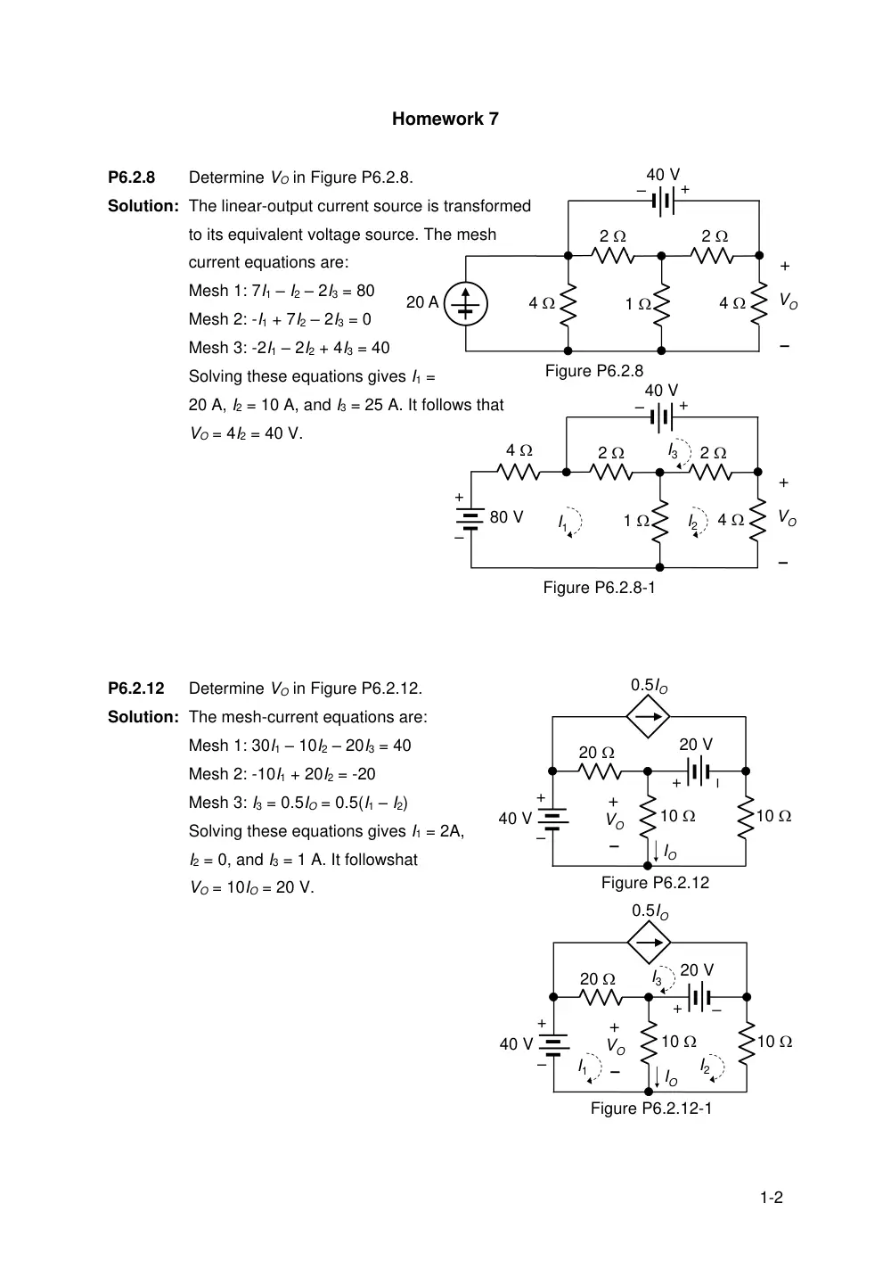
1-2 Homework 7 P6.2.8 Determine VO in Figure P6.2.8. Solution: The linear-output current source is transformed to its equivalent voltage source. The mesh current equations are: Mesh 1: 7I1 – I2 – 2I3 = 80 Mesh 2: -I1 + 7I2 – 2I3 = 0 Mesh 3: -2I1 – 2I2 + 4I3 = 40 Solving these equations gives I1 = 20 A, I2 = 10 A, and I3 = 25 A. It follows that VO = 4I2 = 40 V. P6.2.12 Determine VO in Figure P6.2.12. Solution: The mesh-current equations are: Mesh 1: 30I1 – 10I2 – 20I3 = 40 Mesh 2: -10I1 + 20I2 = -20 Mesh 3: I3 = 0.5IO = 0.5(I1 – I2) Solving these equations gives I1 = 2A, I2 = 0, and I3 = 1 A. It followshat VO = 10IO = 20 V. 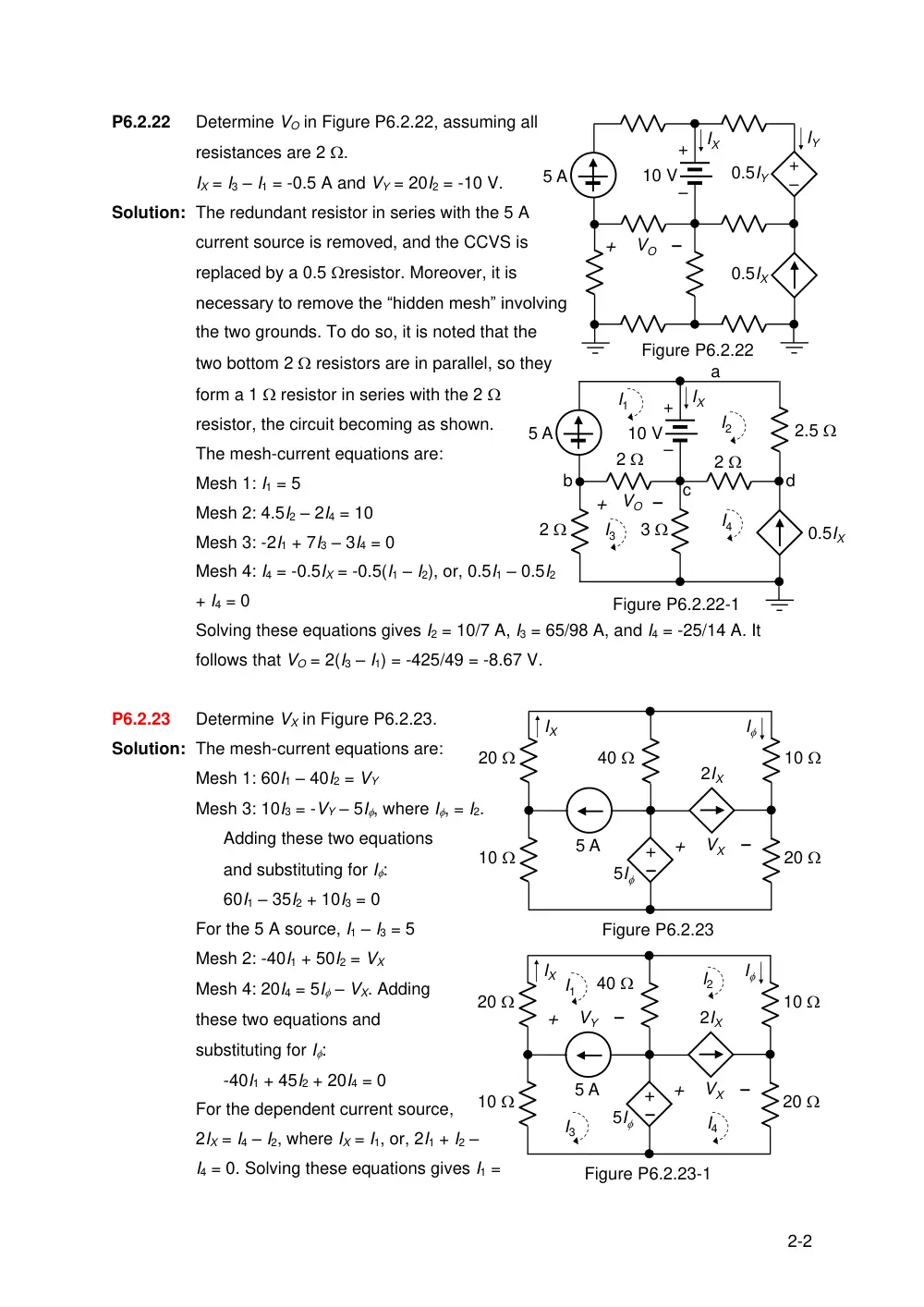20 A 1  2  ` VO + – Figure P6.2.8 4  2  4  + – 40 V 1  2  ` VO + – Figure P6.2.8-1 4  2  4  + – 40 V + – 80 V I1 I2 I3 40 V 20  IO 0.5IO + – VO 10  10  20 V + – + – Figure P6.2.12 40 V 20  IO 0.5IO + – VO 10  10  20 V + – + – Figure P6.2.12-1 I1 I2 I3 2-2 P6.2.22 Determine VO in Figure P6.2.22, assuming all resistances are 2 . IX = I3 – I1 = -0.5 A and VY = 20I2 = -10 V. Solution: The redundant resistor in series with the 5 A current source is removed, and the CCVS is replaced by a 0.5 resistor. Moreover, it is necessary to remove the “hidden mesh” involving the two grounds. To do so, it is noted that the two bottom 2  resistors are in parallel, so they form a 1  resistor in series with the 2  resistor, the circuit becoming as shown. The mesh-current equations are: Mesh 1: I1 = 5 Mesh 2: 4.5I2 – 2I4 = 10 Mesh 3: -2I1 + 7I3 – 3I4 = 0 Mesh 4: I4 = -0.5IX = -0.5(I1 – I2), or, 0.5I1 – 0.5I2 + I4 = 0 Solving these equations gives I2 = 10/7 A, I3 = 65/98 A, and I4 = -25/14 A. It follows that VO = 2(I3 – I1) = -425/49 = -8.67 V. P6.2.23 Determine VX in Figure P6.2.23. Solution: The mesh-current equations are: Mesh 1: 60I1 – 40I2 = VY Mesh 3: 10I3 = -VY – 5I, where I, = I2. Adding these two equations and substituting for I: 60I1 – 35I2 + 10I3 = 0 For the 5 A source, I1 – I3 = 5 Mesh 2: -40I1 + 50I2 = VX Mesh 4: 20I4 = 5I – VX. Adding these two equations and substituting for I: -40I1 + 45I2 + 20I4 = 0 For the dependent current source, 2IX = I4 – I2, where IX = I1, or, 2I1 + I2 – I4 = 0. Solving these equations gives I1 = 0.5IX – + 0.5IY IX IY 10 V 5 A + – + VO – Figure P6.2.22 0.5IX IX 10 V 5 A + – + VO – Figure P6.2.22-1 a b c d 2.5  I1 I4 I2 2  2  2  3  I3 + 10  – 5 A I 5I IX 2IX Figure P6.2.23 20  40  10  20  + VX – + 10  – 5 A I 5I IX 2IX Figure P6.2.23-1 20  40  10  20  + VX – I1 I2 I3 I4 + VY – 3-2 5/7 A, I2 = 0, I3 = -30/7, and I4 = 10/7. It follows that VX = 40(I2 – I1) +10I2 = -40I1 = -200/7 = -28.57 V. 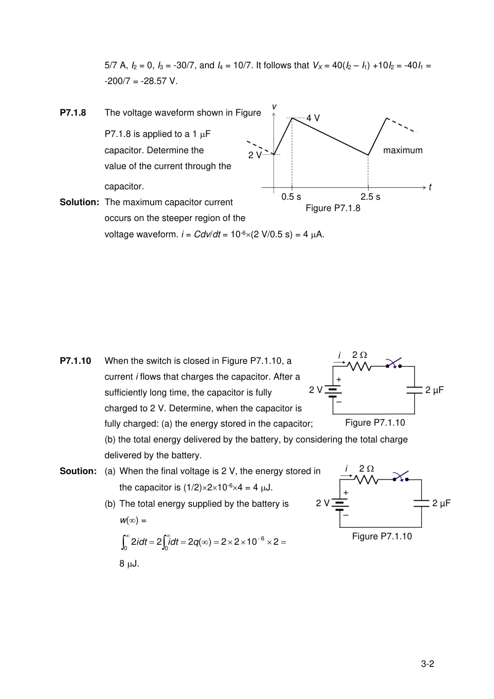P7.1.8 The voltage waveform shown in Figure P7.1.8 is applied to a 1 F capacitor. Determine the maximum value of the current through the capacitor. Solution: The maximum capacitor current occurs on the steeper region of the voltage waveform. i = Cdv/dt = 10-6(2 V/0.5 s) = 4 A. P7.1.10 When the switch is closed in Figure P7.1.10, a current i flows that charges the capacitor. After a sufficiently long time, the capacitor is fully charged to 2 V. Determine, when the capacitor is fully charged: (a) the energy stored in the capacitor; (b) the total energy delivered by the battery, by considering the total charge delivered by the battery. Soution: (a) When the final voltage is 2 V, the energy stored in the capacitor is (1/2)210-64 = 4 J. (b) The total energy supplied by the battery is w() =              0 6 0 2 2 10 2 2 ( ) 2 2 q idt idt 8 J. 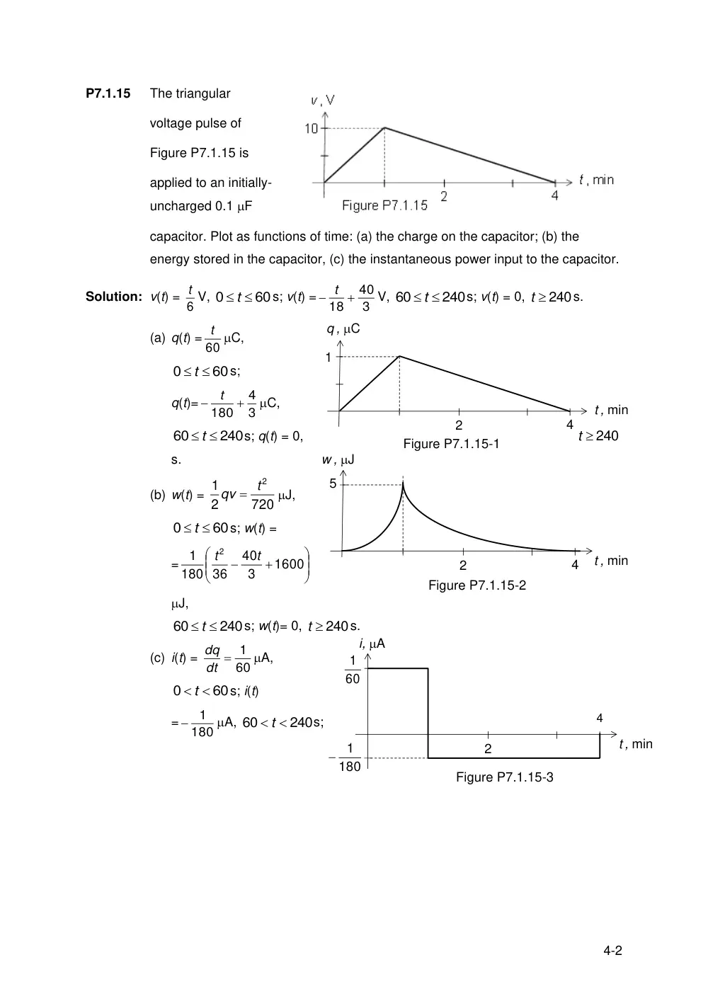t v 0.5 s 2.5 s 2 V 4 V Figure P7.1.8 2 µF 2 V + – 2  Figure P7.1.10 i 2 µF 2 V + – 2  Figure P7.1.10 i 4-2 P7.1.15 The triangular voltage pulse of Figure P7.1.15 is applied to an initially- uncharged 0.1 F capacitor. Plot as functions of time: (a) the charge on the capacitor; (b) the energy stored in the capacitor, (c) the instantaneous power input to the capacitor. Solution: v(t) = 6 t V, 60 0  t  s; v(t) = 3 40 18   t V, 240 60  t  s; v(t) = 0, t  240 s. (a) q(t) = 60 t C, 60 0  t  s; q(t)= 3 4  180  t C, 240 60  t  s; q(t) = 0,  240 t s. (b) w(t) = 720 2 1 2t qv  J, 60 0  t  s; w(t) = =         1600 3 40 36 180 1 2 t t J, 240 60  t  s; w(t)= 0, t  240 s. (c) i(t) = 60 dt  1 dq A, 60 0  t  s; i(t) = 180 1  A, 240 60  t  s; 4 t , min q , C 1 2 Figure P7.1.15-1 4 t , min w , J 5 2 Figure P7.1.15-2 4 t , min i, A 2 60 1 180 1  Figure P7.1.15-3 5-2 i(t)= 0, t  240 s, where 60 1 A may also be expressed as 1 C/min. 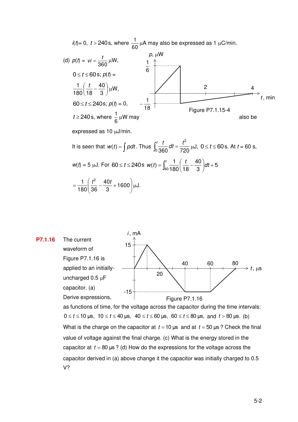(d) p(t) = 360 t vi  W, 60 0  t  s; p(t) =        3 40 18 180 1 t W, 240 60  t  s; p(t) = 0, t  240 s, where 6 1 W may also be expressed as 10 J/min. It is seen that   pdt t w ) ( . Thus   t t dt t 0 2 720 360 J, 60 0  t  s. At t = 60 s, w(t) = 5 J. For 240 60  t  s           t dt t t w 60 5 3 40 18 180 1 ( )          1600 3 40 36 180 1 2 t t J. 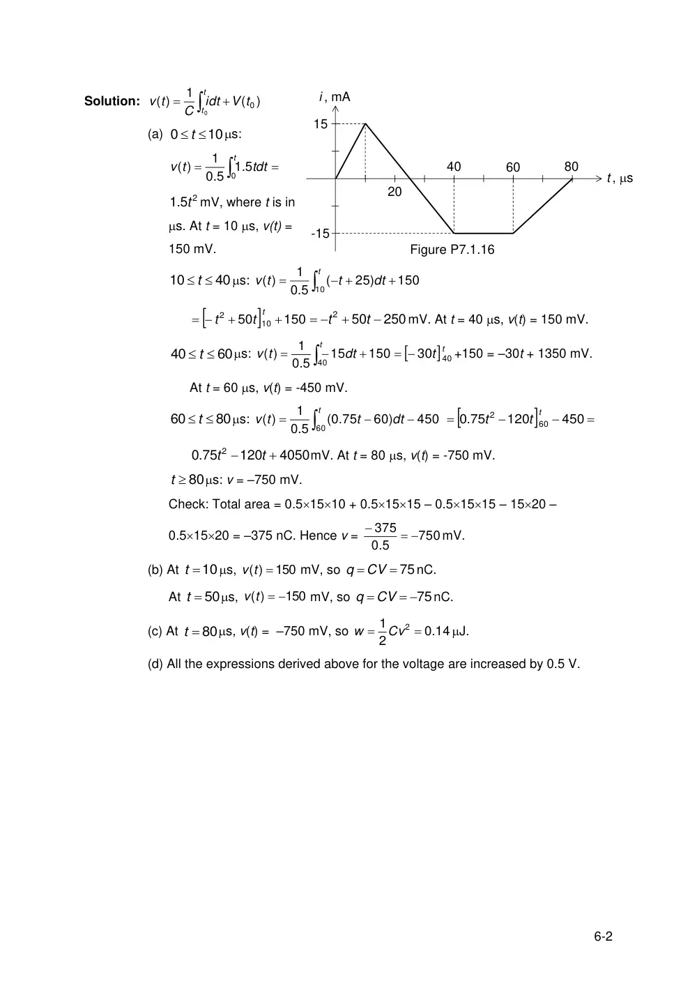P7.1.16 The current waveform of Figure P7.1.16 is applied to an initially- uncharged 0.5 F capacitor. (a) Derive expressions, as functions of time, for the voltage across the capacitor during the time intervals: 10 μs, 0  t  40 μs, 10  t  60 μs, 40  t  80 μs, 60  t  and t  80 μs. (b) What is the charge on the capacitor at t  10 μs and at t  50 μs ? Check the final value of voltage against the final charge. (c) What is the energy stored in the capacitor at t  80 μs ? (d) How do the expressions for the voltage across the capacitor derived in (a) above change it the capacitor was initially charged to 0.5 V? 4 t , min p, W 2 6 1 18 1  Figure P7.1.15-4 i , mA t , s 15 20 40 60 80 -15 Figure P7.1.16 6-2 Solution: ) ( 1 ( ) 0 0 V t idt C t v t t    (a) 10 0  t  s:    t tdt t v 0 5 1. 0.5 1 ( ) .5 2 1 t mV, where t is in s. At t = 10 s, v(t) = 150 mV. 40 10  t  s:      t dt t t v 10 150 25) ( 0.5 1 ( )   150 50 10 2     t t t 250 50 2     t t mV. At t = 40 s, v(t) = 150 mV. 60 40  t  s:     t dt t v 40 150 15 0.5 1 ( )  t t   30 40 +150 = –30t + 1350 mV. At t = 60 s, v(t) = -450 mV. 80 60  t  s:     t dt t t v 60 450 60) (0.75 0.5 1 ( )       450 120 .75 0 60 2 t t t 4050 120 0.75 2   t t mV. At t = 80 s, v(t) = -750 mV. t  80 s: v = –750 mV. Check: Total area = 0.51510 + 0.51515 – 0.51515 – 1520 – 0.51520 = –375 nC. Hence v = 750 0.5 375    mV. (b) At t 10 s, 150 ( ) v t  mV, so q  CV  75 nC. At t  50 s, 150 ( ) v t   mV, so q CV  75 nC. (c) At t  80 s, v(t) = –750 mV, so 0.14 2 1 2   Cv w J. (d) All the expressions derived above for the voltage are increased by 0.5 V. i , mA t , s 15 20 40 60 80 -15 Figure P7.1.16