EECE 290 Homework 2 with Solution, Spring 2011

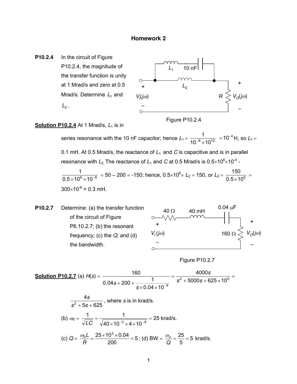
1 Homework 2 P10.2.4 In the circuit of Figure P10.2.4, the magnitude of the transfer function is unity at 1 Mrad/s and zero at 0.5 Mrad/s. Determine 1 L and 2 L . Solution P10.2.4 At 1 Mrad/s, L1 is in series resonance with the 10 nF capacitor; hence L1 = 12 8 10 10 1 − × =10−4 H, so L1 = 0.1 mH. At 0.5 Mrad/s, the reactance of L1 and C is capacitive and is in parallel resonance with L2. The reactance of L1 and C at 0.5 Mrad/s is 0.5×106×10-4 - 8 6 10 0.5 10 1 − × × = 50 – 200 = -150; hence, 0.5×106× L2 = 150, or L2 = 0.5 106 150 × = 300×10-6 = 0.3 mH. P10.2.7 Determine: (a) the transfer function of the circuit of Figure P6.10.2.7; (b) the resonant frequency; (c) the Q; and (d) the bandwidth. Solution P10.2.7 (a) H(s) = = × × + + 0.04 10−6 1 200 .04 0 160 s s = × + + 6 2 10 625 5000 4000 s s s 625 5 4 2 s + s + s , where s is in krad/s. (b) ω0 = 8 3 4 10 10 40 1 1 − − × × × = LC = 25 krad/s. (c) Q = 5 200 0.04 10 25 3 0 = × × = R ω L ; (d) BW = 5 5 = 25 = Q ωo krad/s. 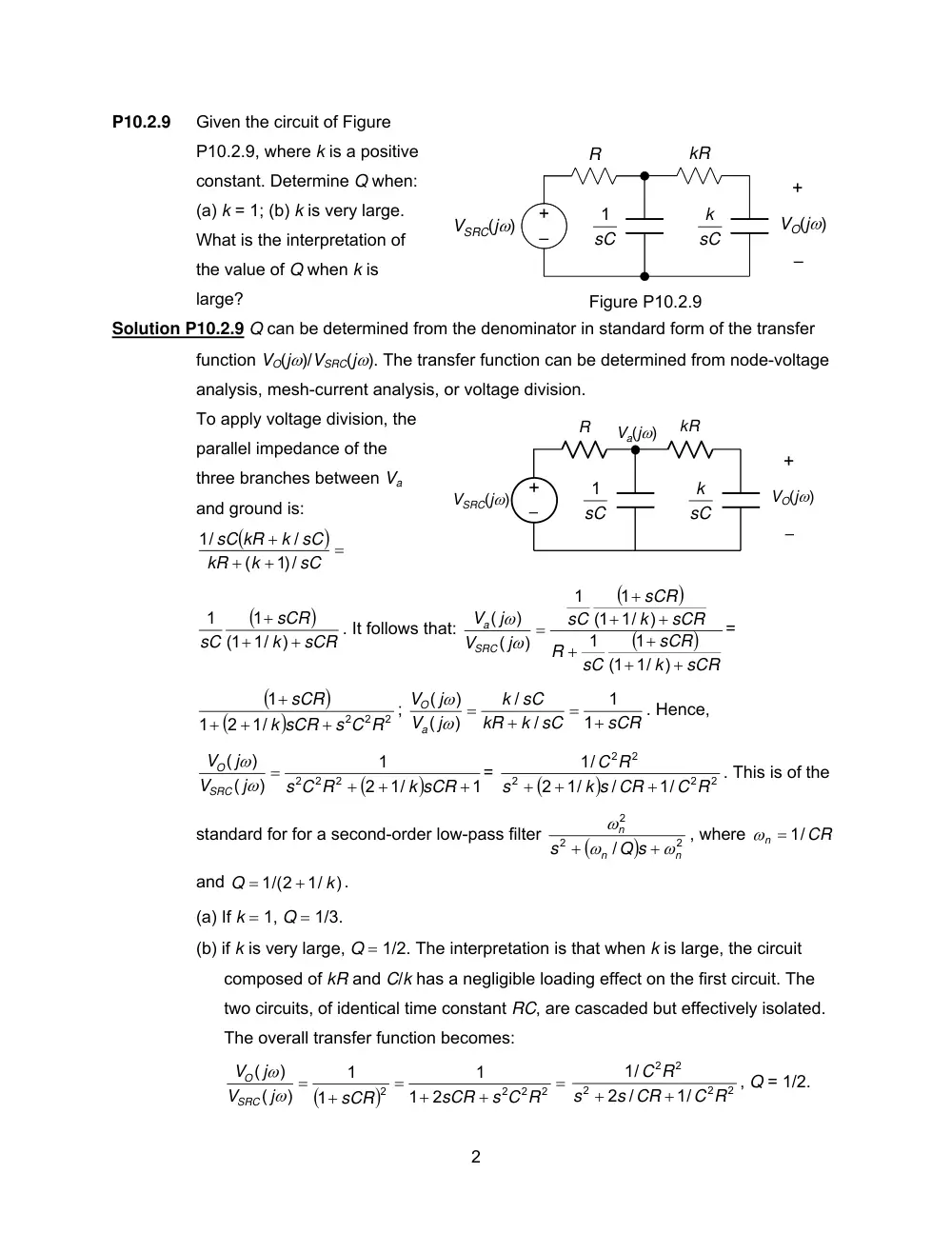Figure P10.2.4 10 nF L1 + – VO(jω) + – VI(jω) R L2 Figure P10.2.7 40 Ω 0.04 μF 40 mH 160 Ω + – VO(jω) + – VI (jω) 2 P10.2.9 Given the circuit of Figure P10.2.9, where k is a positive constant. Determine Q when: (a) k = 1; (b) k is very large. What is the interpretation of the value of Q when k is large? Solution P10.2.9 Q can be determined from the denominator in standard form of the transfer function VO(jω)/VSRC(jω). The transfer function can be determined from node-voltage analysis, mesh-current analysis, or voltage division. To apply voltage division, the parallel impedance of the three branches between Va and ground is: ( ) = + + + sC k kR k sC sC kR /)1 ( / 1/ ( ) sCR k sCR sC + + + ) (1 1/ 1 1 . It follows that: ( ) ( ) sCR k sCR sC R sCR k sCR sC j V j V SRC a + + + + + + + = ) (1 1/ 1 1 ) (1 1/ 1 1 ) ( ) ( ω ω = ( ) ( ) 2 2 2 1/ 2 1 1 s C R k sCR sCR + + + + ; sCR k sC kR k sC j V j V a O + = + = 1 1 / / ) ( ) ( ω ω . Hence, ( ) 1 1/ 2 1 ) ( ) ( 2 2 2 + + + = k sCR s C R j V j V SRC O ω ω = ( ) 2 2 2 2 2 1/ / 1/ 2 1/ C R k s CR s C R + + + . This is of the standard for for a second-order low-pass filter ( ) 2 2 2 / n n n Q s s ω ω ω + + , where CR n = 1/ ω and ) 1/ 1/(2 k Q + = . (a) If k = 1, Q = 1/3. (b) if k is very large, Q = 1/2. The interpretation is that when k is large, the circuit composed of kR and C/k has a negligible loading effect on the first circuit. The two circuits, of identical time constant RC, are cascaded but effectively isolated. The overall transfer function becomes: ( ) = + + = + = 2 2 2 2 2 1 1 1 1 ) ( ) ( s C R sCR sCR j V j V SRC O ω ω 2 2 2 2 2 1/ 2 / 1/ C R s CR s C R + + , Q = 1/2. 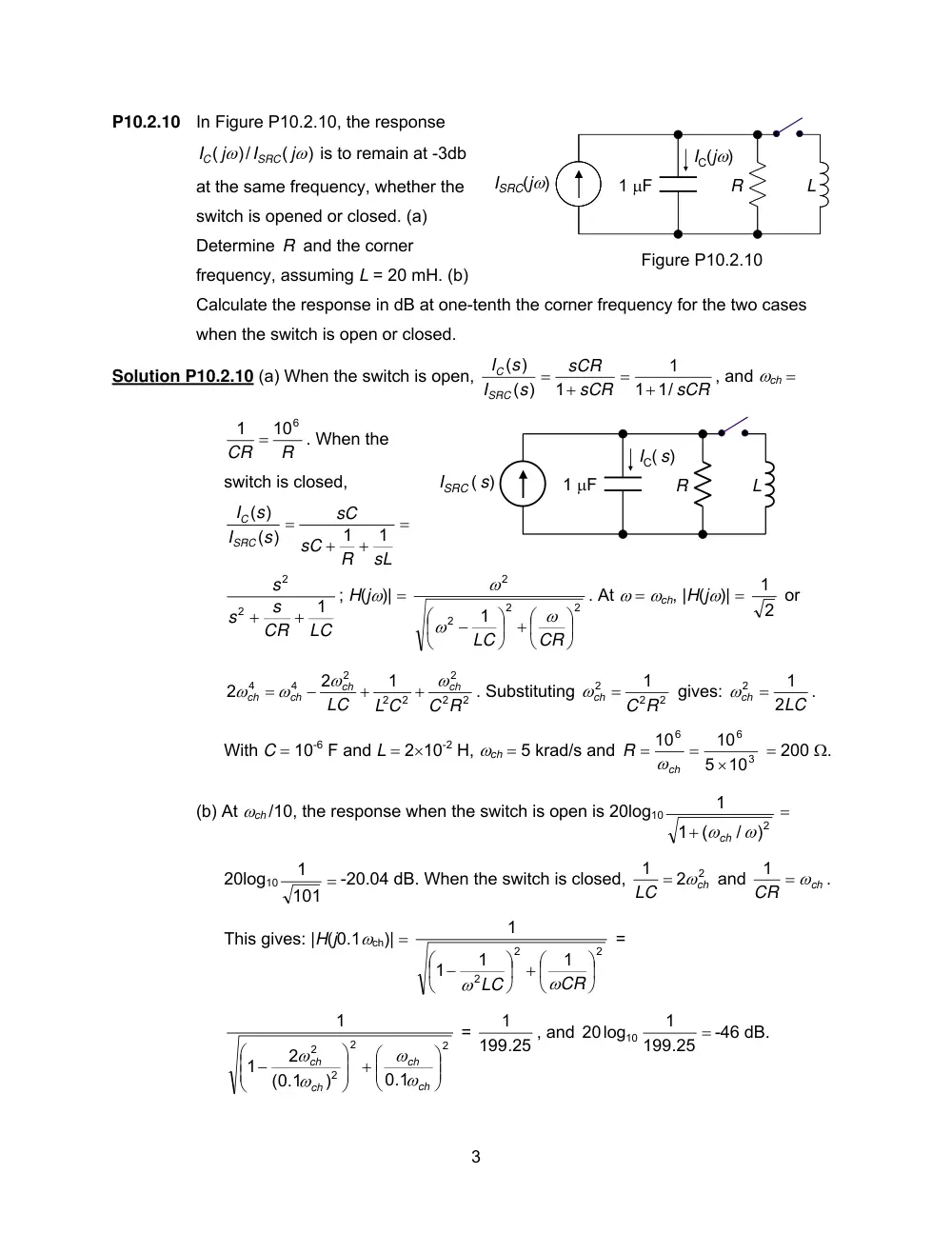R kR sC 1 sC k Figure P10.2.9 + – VO(jω) – + VSRC(jω) R kR sC 1 sC k + – VO(jω) – + VSRC(jω) Va(jω) 3 P10.2.10 In Figure P10.2.10, the response ) ( /) ( ω ω j I j I SRC C is to remain at -3db at the same frequency, whether the switch is opened or closed. (a) Determine R and the corner frequency, assuming L = 20 mH. (b) Calculate the response in dB at one-tenth the corner frequency for the two cases when the switch is open or closed. Solution P10.2.10 (a) When the switch is open, sCR sCR sCR s I s I SRC C 1/ 1 1 1 ( ) ( ) + = + = , and ωch = R CR 1 = 106 . When the switch is closed, = + + = sL R sC sC s I s I SRC C 1 1 ( ) ) ( LC CR s s s 1 2 2 + + ; H(jω)| = 2 2 2 2 1 ⎟ ⎠ ⎞ ⎜ ⎝ ⎟ + ⎛ ⎠ ⎞ ⎜ ⎝ ⎛ − CR LC ω ω ω . At ω = ωch, |H(jω)| = 2 1 or 2 2 2 2 2 2 4 4 1 2 2 C R L C LC ch ch ch ch ω ω ω ω + + − = . Substituting 2 2 2 1 C R ωch = gives: LC ch 2 1 ω2 = . With C = 10-6 F and L = 2×10-2 H, ωch = 5 krad/s and 3 6 6 10 5 10 10 × = = ch R ω = 200 Ω. (b) At ωch /10, the response when the switch is open is 20log10 2) / ( 1 1 ωch ω + = 20log10 = 101 1 -20.04 dB. When the switch is closed, 2 2 1 ch LC = ω and ch CR 1 = ω . This gives: |H(j0.1ωch)| = 2 2 2 1 1 1 1 ⎟ ⎠ ⎞ ⎜ ⎝ ⎟ + ⎛ ⎠ ⎞ ⎜ ⎝ ⎛ − CR LC ω ω = 2 2 2 2 0.1 ) (0.1 2 1 1 ⎟⎟ ⎠ ⎞ ⎜⎜ ⎝ ⎟⎟ + ⎛ ⎠ ⎞ ⎜⎜ ⎝ ⎛ − ch ch ch ch ω ω ω ω = 199.25 1 , and 199.25 = 1 20log 10 -46 dB. 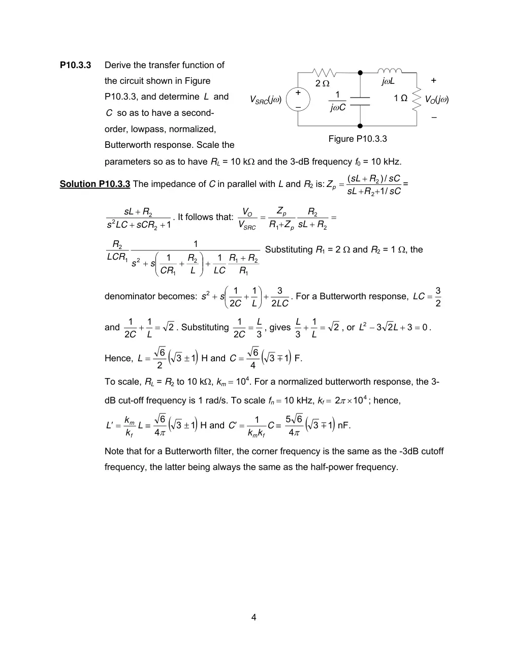R ISRC ( s) L 1 μF IC( s) R ISRC(jω) L 1 μF IC(jω) Figure P10.2.10 4 P10.3.3 Derive the transfer function of the circuit shown in Figure P10.3.3, and determine L and C so as to have a second- order, lowpass, normalized, Butterworth response. Scale the parameters so as to have RL = 10 kΩ and the 3-dB frequency f0 = 10 kHz. Solution P10.3.3 The impedance of C in parallel with L and R2 is: sC sL R sC R sL Zp 1/ /) ( 2 2 + + + = = 1 2 2 2 + + + sCR s LC R sL . It follows that: = + + = 2 2 1 R sL R Z R Z V V p p SRC O 1 2 1 2 1 2 1 2 1 1 1 R R R LC L R s CR LCR s R + ⎟⎟ + ⎠ ⎞ ⎜⎜ ⎝ ⎛ + + Substituting R1 = 2 Ω and R2 = 1 Ω, the denominator becomes: s2 + LC L C s 2 3 1 2 1 ⎟ + ⎠ ⎞ ⎜ ⎝ ⎛ + . For a Butterworth response, 2 LC = 3 and 2 1 2 1 C + L = . Substituting 3 2 1 C = L , gives 2 1 3 L + L = , or 0 3 2 3 2 = + − L L . Hence, ( )1 3 2 6 ± L = H and ( )1 3 4 6 m C = F. To scale, RL = R2 to 10 kΩ, km = 104. For a normalized butterworth response, the 3- dB cut-off frequency is 1 rad/s. To scale fn = 10 kHz, kf = 2 ×104 π ; hence, ≡ ′ = L k k L f m ( )1 3 4 6 ± π H and k k C C f m 1 ′ = ≡ ( )1 3 4 5 6 m π nF. Note that for a Butterworth filter, the corner frequency is the same as the -3dB cutoff frequency, the latter being always the same as the half-power frequency. 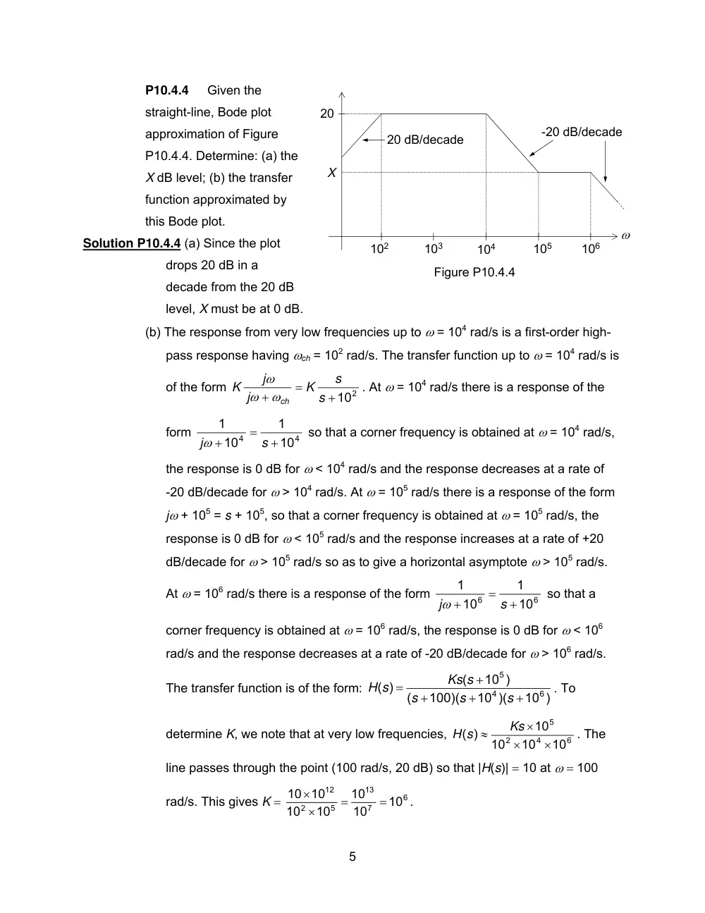Figure P10.3.3 + – VO(jω) 2 Ω – + VSRC(jω) jωC 1 jωL 1 Ω 5 P10.4.4 Given the straight-line, Bode plot approximation of Figure P10.4.4. Determine: (a) the X dB level; (b) the transfer function approximated by this Bode plot. Solution P10.4.4 (a) Since the plot drops 20 dB in a decade from the 20 dB level, X must be at 0 dB. (b) The response from very low frequencies up to ω = 104 rad/s is a first-order high- pass response having ωch = 102 rad/s. The transfer function up to ω = 104 rad/s is of the form +102 = + s s K j j K ωch ω ω . At ω = 104 rad/s there is a response of the form 4 4 10 1 10 1 + = + s jω so that a corner frequency is obtained at ω = 104 rad/s, the response is 0 dB for ω < 104 rad/s and the response decreases at a rate of -20 dB/decade for ω > 104 rad/s. At ω = 105 rad/s there is a response of the form jω + 105 = s + 105, so that a corner frequency is obtained at ω = 105 rad/s, the response is 0 dB for ω < 105 rad/s and the response increases at a rate of +20 dB/decade for ω > 105 rad/s so as to give a horizontal asymptote ω > 105 rad/s. At ω = 106 rad/s there is a response of the form 6 6 10 1 10 1 + = + s jω so that a corner frequency is obtained at ω = 106 rad/s, the response is 0 dB for ω < 106 rad/s and the response decreases at a rate of -20 dB/decade for ω > 106 rad/s. The transfer function is of the form: 10 ) 10 )( 100)( ( 10 ) ( ) ( 6 4 5 + + + + = s s s Ks s H s . To determine K, we note that at very low frequencies, 6 4 2 5 10 10 10 10 ( ) × × × ≈ Ks H s . The line passes through the point (100 rad/s, 20 dB) so that |H(s)| = 10 at ω = 100 rad/s. This gives K = 6 7 13 5 2 12 10 10 10 10 10 10 10 = = × × . Figure P10.4.4 ω 102 103 104 105 106 20 X -20 dB/decade 20 dB/decade