EECE 290 Homework 3, Spring 2015

Figure P14.2.6 C L + – VO (j) 0.1 mA R Figure P14.2.7 1 mH VSRC (j) 1 k 1 F – + 0.9VSRCj) – + Figure P14.2.7 VSRC(j) 1 k – + – + IC(j) jL 1/jC 0.9VSRC(j) + 0.1VSRC(j) – Homework 3 P14.2.6 Determine R, L, and C In Figure P14.2.6 so that the maximum response is 1 V, 0 = 100 krad/s, and BW = 4 krad/s. Short Solution: maximum response occurs when the combined impedance of L and C is infinite. The source current flows through R. so that: R(0.1 mA) = 1 V, which gives R = 10 k. From the given data, Q = 0/BW = 100/4 = 25 = 0CR, so that C = 25/(0R) = 25/(105104) = 2510-9 F  25 nF. Since , or, H  4 mH. P14.2.7 Determine 0 and Q in Figure P14.2.7. Solution: The first step is to account for the dependent source. The voltage across the capacitor is 0.1 VSRC(j). Hence, (0.1VSRC(j))(jC) = VSRC(j)j(0.1C). In other words, the capacitor C in series with the dependent source is equivalent to a capacitor 0.1C. This is in accordance with the source absorption theorem, for the current through the dependent source is VSRC(j)j(0.1C). Dividing this by the voltage 0.9VSRC, the dependent source is equivalent to an admittance jC/9, or a capacitor C/9. This capacitor in series with C gives a capacitance C(C/9)/(C + C/9) = 0.1C. + – VO ( j) 750  50 H 20 nF VSRC ( j) – + Figure P14.2.10 + – VO ( j) 40 k 100 mH 100 nF VSRC ( j) – + Figure P14.2.12 10 k It follows that rad/s  100 krad/s. Q = 0RC = 10510-7103 = 10. 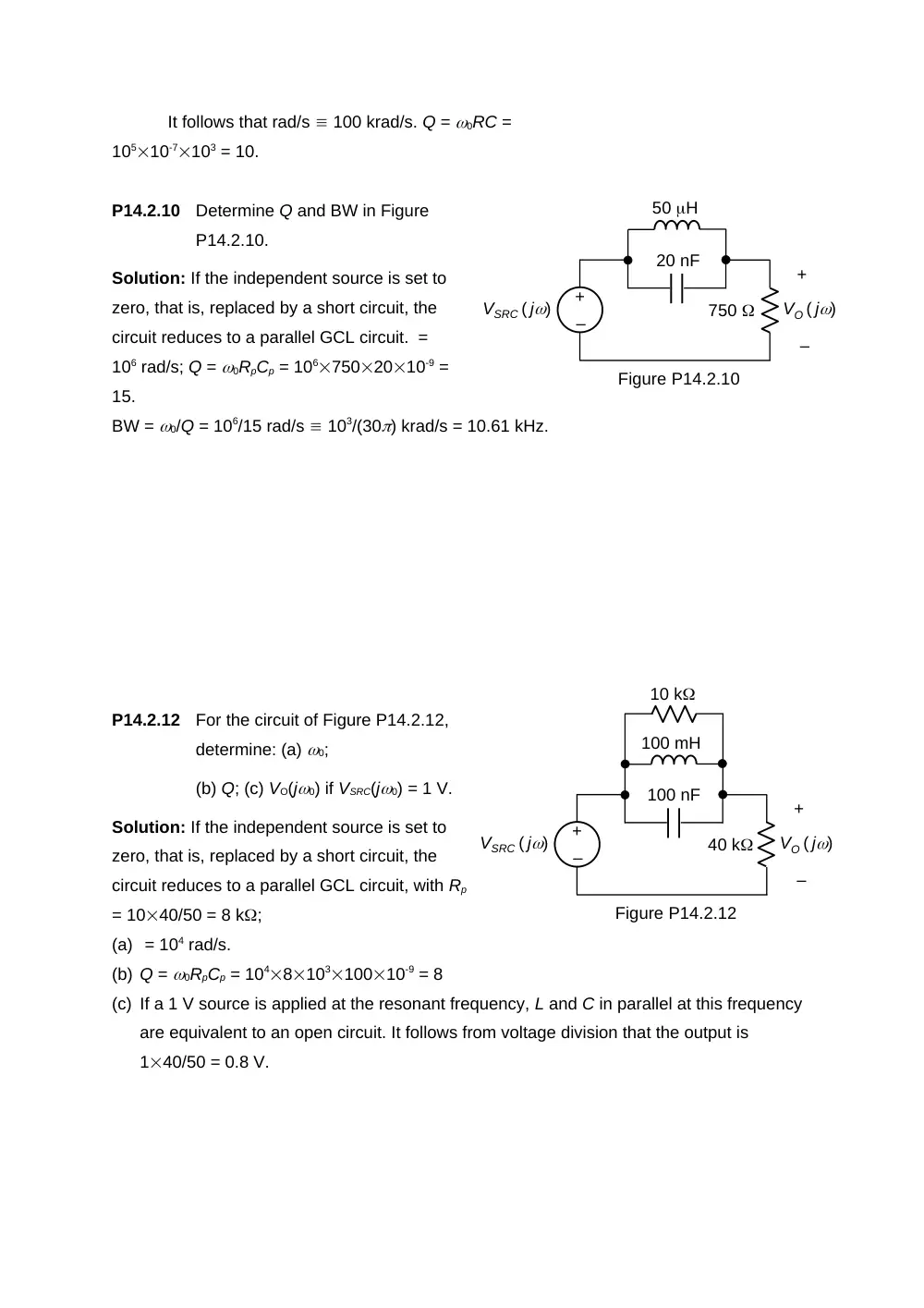P14.2.10 Determine Q and BW in Figure P14.2.10. Solution: If the independent source is set to zero, that is, replaced by a short circuit, the circuit reduces to a parallel GCL circuit. = 106 rad/s; Q = 0RpCp = 1067502010-9 = 15. BW = 0/Q = 106/15 rad/s  103/(30) krad/s = 10.61 kHz. P14.2.12 For the circuit of Figure P14.2.12, determine: (a) 0; (b) Q; (c) VO(j0) if VSRC(j0) = 1 V. Solution: If the independent source is set to zero, that is, replaced by a short circuit, the circuit reduces to a parallel GCL circuit, with Rp = 1040/50 = 8 k; (a) = 104 rad/s. (b) Q = 0RpCp = 104810310010-9 = 8 (c) If a 1 V source is applied at the resonant frequency, L and C in parallel at this frequency are equivalent to an open circuit. It follows from voltage division that the output is 140/50 = 0.8 V. 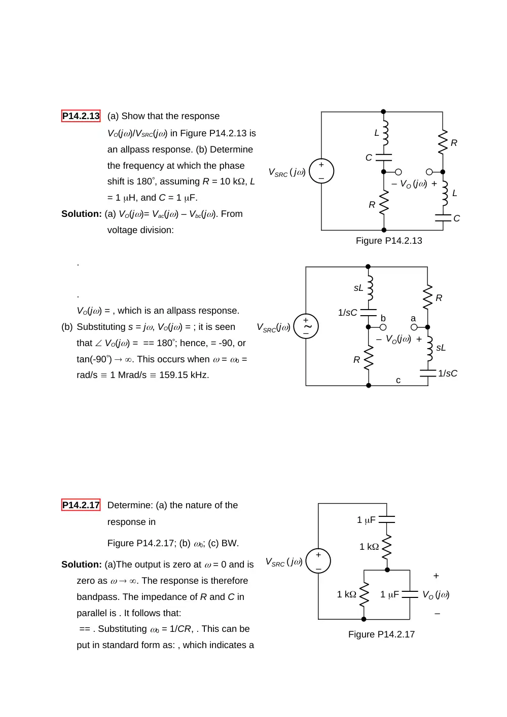Figure P14.2.13 – + VSRC ( j) R L + – VO (j) C R L C Figure P14.2.17 1 k + – VO (j) 1 F 1 F – + VSRC ( j) 1 k – + R sL + – VO(j) 1/sC R  a b c sL 1/sC VSRC(j) P14.2.13 (a) Show that the response VO(j)/VSRC(j) in Figure P14.2.13 is an allpass response. (b) Determine the frequency at which the phase shift is 180, assuming R = 10 k, L = 1 H, and C = 1 F. Solution: (a) VO(j)= Vac(j) – Vbc(j). From voltage division: . . VO(j) = , which is an allpass response. (b) Substituting s = j, VO(j) = ; it is seen that  VO(j) = == 180; hence, = -90, or tan(-90)  . This occurs when  = 0 = rad/s  1 Mrad/s  159.15 kHz. P14.2.17 Determine: (a) the nature of the response in Figure P14.2.17; (b) 0; (c) BW. Solution: (a)The output is zero at  = 0 and is zero as   . The response is therefore bandpass. The impedance of R and C in parallel is . It follows that: == . Substituting 0 = 1/CR, . This can be put in standard form as: , which indicates a  20log10|H(j)|, dB 0 -20 2 25 250  20log10|H(j)|, dB 0 20 -20 2 25 250 Figure P14.3.8 Q = 1/3 and a maximum gain of 1/3. (b) 0 = 1/CR = 1/(10-6103) = 103 rad/s  1 krad/s. (c) BW = 0/Q = 1/(1/3) = 3 krad/s. P14.3.3 Given . Determine the smaller 3-db cutoff frequency. Short Solution: , BW = 50 = 2 – 1; ; = 0; ; 1 = 40 rad/s. P14.3.8 Determine the transfer function whose asymptotic Bode magnitude plot is shown in Figure P14.3.8. Solution: The first part, as shown, is a highpass response of corner frequency 2 rad/s. The transfer function is: =, and . If   , and 20log10; if   0, , and 20log10 20log10() – 20log10(2), which is the equation of the LF asymptote. The second part is the mirror image, with respect to the horizontal axis, of the low pass response shown, having a corner frequency 25 rad/s. The transfer function is: =, and ; if   0, ; 20log10; if   , , and 20log1020log10(25) – 20log10(),which is the equation of the HF asymptote. The transfer function of the mirror image with respect to the horizontal axis is the reciprocal on a log scale. The transfer function of the given part is therefore =. The overall Bode plots is the sum of the Bode plots of the two parts on a log scale, which corresponds to the product of the  20log10|H(j)|, dB 0 -20 2 25 250 transfer functions, that is: .