MATH 218 Notes Final Exam NOTES, Spring 2012

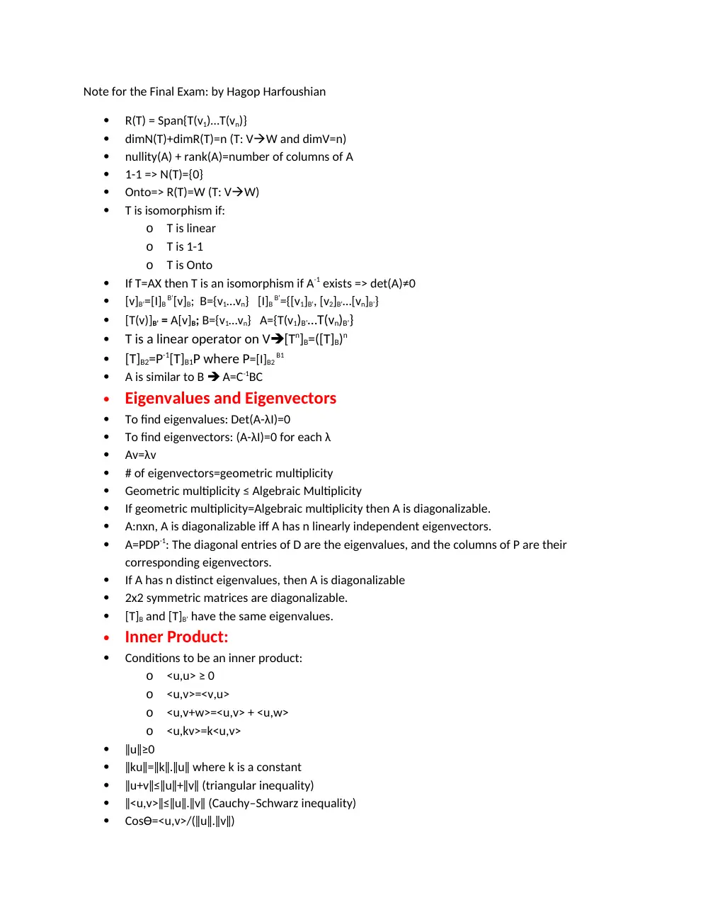
Note for the Final Exam: by Hagop Harfoushian  R(T) = Span{T(v1)…T(vn)}  dimN(T)+dimR(T)=n (T: VW and dimV=n)  nullity(A) + rank(A)=number of columns of A  1-1 => N(T)={0}  Onto=> R(T)=W (T: VW)  T is isomorphism if: o T is linear o T is 1-1 o T is Onto  If T=AX then T is an isomorphism if A-1 exists => det(A)≠0  [v]B’=[I]B B’[v]B; B={v1…vn} [I]B B’={[v1]B’, [v2]B’…[vn]B’}  [T(v)]B’ = A[v]B; B={v1…vn} A={T(v1)B’…T(vn)B’}  T is a linear operator on V[Tn]B=([T]B)n  [T]B2=P-1[T]B1P where P=[I]B2 B1  A is similar to B  A=C-1BC  Eigenvalues and Eigenvectors  To find eigenvalues: Det(A-λI)=0  To find eigenvectors: (A-λI)=0 for each λ  Av=λv  # of eigenvectors=geometric multiplicity  Geometric multiplicity ≤ Algebraic Multiplicity  If geometric multiplicity=Algebraic multiplicity then A is diagonalizable.  A:nxn, A is diagonalizable iff A has n linearly independent eigenvectors.  A=PDP-1: The diagonal entries of D are the eigenvalues, and the columns of P are their corresponding eigenvectors.  If A has n distinct eigenvalues, then A is diagonalizable  2x2 symmetric matrices are diagonalizable.  [T]B and [T]B’ have the same eigenvalues.  Inner Product:  Conditions to be an inner product: o <u,u> ≥ 0 o <u,v>=<v,u> o <u,v+w>=<u,v> + <u,w> o <u,kv>=k<u,v>  ǁuǁ≥0  ǁkuǁ=ǁkǁ.ǁuǁ where k is a constant  ǁu+vǁ≤ǁuǁ+ǁvǁ (triangular inequality)  ǁ<u,v>ǁ≤ǁuǁ.ǁvǁ (Cauchy–Schwarz inequality)  Cosϴ=<u,v>/(ǁuǁ.ǁvǁ)  ǁuǁ=√(<u,u>)  D(u,v)= ǁu-vǁ (distance between u and v)  Col(A):  put A in REF, then take the pivot columns from the original matrix (not from the REF)  Row(A): put A in REF, then take the pivot rows from the REF matrix  Ci=<vi , v>  Proju v= (<u,v>/ǁvǁ2). V  U- Proju v and V are orthogonal  Gran Schmidt process: o W1=V1 o W2=V2- Projv2 w1 o W3=V3= Projv3 w1- Projv3 w2 o …  W ⊥is a subspace  W⊥∩W={0}  dimV= dimW⊥+ dimW  N(At)= y/Aty=0 (definition)  N(A)= x/Ax=0  N(A)=(rowA) ⊥  N(At)=(colA) ⊥  Projv W=Σ(<b,wi>/ǁwiǁ2). Wi Where W is an Orthogonal basis  Ax=b is inconsistent if b ∉ col(A)  Ax= Projv Col(A) is the closest vector for the system to be consistent  Least mean square solutions  ẍ is the least mean square solution  Procedure to find ẍ o Find a basis for col(A) (by placing in REF and taking the pivot columns from the original matrix) o Use Gran Schmidt to find orthogonal matrix o Find Projv W=Σ(<b,wi>/ǁwiǁ2 where W=col(A) o Solve A ẍ= Projv W  Procedure 2 to find ẍ o Solve AtAx=Atb  A ẍ= Projv Col(A) PREPARED BY HAGOP HARFOUSHIAN