MECH 340 Lecture, Fall 2006

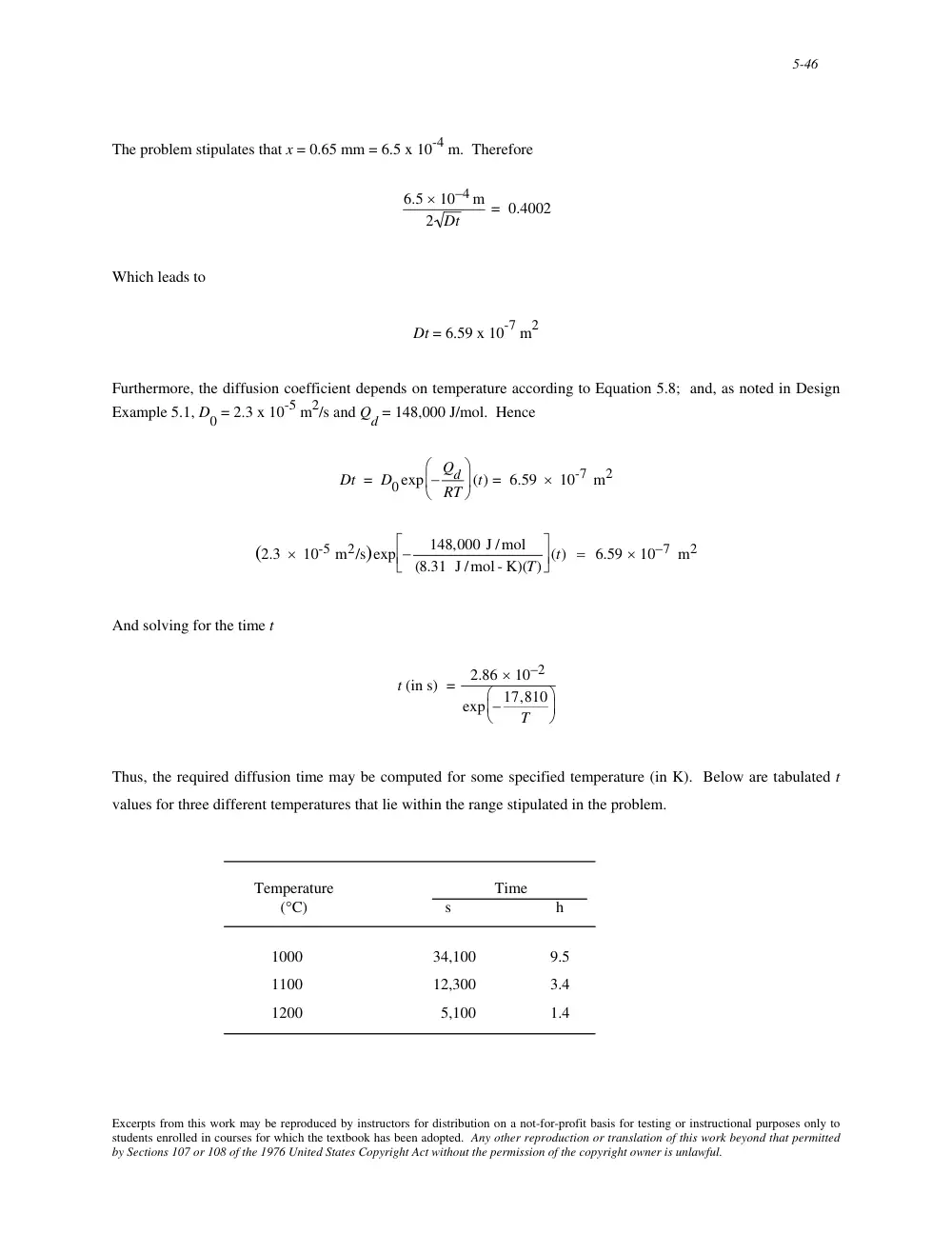
5-46 The problem stipulates that x = 0.65 mm = 6.5 x 10-4 m. Therefore 6.5 × 10−4 m 2 Dt = 0.4002 Which leads to Dt = 6.59 x 10-7 m2 Furthermore, the diffusion coefficient depends on temperature according to Equation 5.8; and, as noted in Design Example 5.1, D0 = 2.3 x 10-5 m2/s and Qd = 148,000 J/mol. Hence Dt = D0exp − Qd RT ⎛ ⎝ ⎜ ⎞ ⎠ ⎟ (t) = 6.59 × 10-7 m2 (2.3 × 10-5 m2/s)exp − 148,000 J /mol (8.31 J /mol - K)(T) ⎡ ⎣ ⎢ ⎤ ⎦ ⎥ (t) = 6.59 × 10−7 m2 And solving for the time t t (in s) = 2.86 × 10−2 exp − 17,810 T ⎛ ⎝ ⎜ ⎞ ⎠ ⎟ Thus, the required diffusion time may be computed for some specified temperature (in K). Below are tabulated t values for three different temperatures that lie within the range stipulated in the problem. Temperature Time (°C) s h 1000 34,100 9.5 1100 12,300 3.4 1200 5,100 1.4 Excerpts from this work may be reproduced by instructors for distribution on a not-for-profit basis for testing or instructional purposes only to students enrolled in courses for which the textbook has been adopted. Any other reproduction or translation of this work beyond that permitted by Sections 107 or 108 of the 1976 United States Copyright Act without the permission of the copyright owner is unlawful. 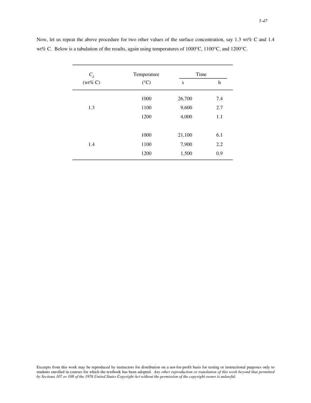5-47 Now, let us repeat the above procedure for two other values of the surface concentration, say 1.3 wt% C and 1.4 wt% C. Below is a tabulation of the results, again using temperatures of 1000°C, 1100°C, and 1200°C. Cs Temperature Time (wt% C) (°C) s h 1000 26,700 7.4 1.3 1100 9,600 2.7 1200 4,000 1.1 1000 21,100 6.1 1.4 1100 7,900 2.2 1200 1,500 0.9 Excerpts from this work may be reproduced by instructors for distribution on a not-for-profit basis for testing or instructional purposes only to students enrolled in courses for which the textbook has been adopted. Any other reproduction or translation of this work beyond that permitted by Sections 107 or 108 of the 1976 United States Copyright Act without the permission of the copyright owner is unlawful. 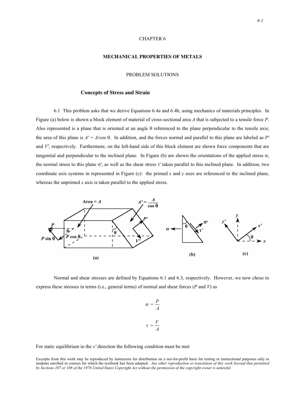6-1 CHAPTER 6 MECHANICAL PROPERTIES OF METALS PROBLEM SOLUTIONS Concepts of Stress and Strain 6.1 This problem asks that we derive Equations 6.4a and 6.4b, using mechanics of materials principles. In Figure (a) below is shown a block element of material of cross-sectional area A that is subjected to a tensile force P. Also represented is a plane that is oriented at an angle θ referenced to the plane perpendicular to the tensile axis; the area of this plane is A' = A/cos θ. In addition, and the forces normal and parallel to this plane are labeled as P' and V', respectively. Furthermore, on the left-hand side of this block element are shown force components that are tangential and perpendicular to the inclined plane. In Figure (b) are shown the orientations of the applied stress σ, the normal stress to this plane σ', as well as the shear stress τ' taken parallel to this inclined plane. In addition, two coordinate axis systems in represented in Figure (c): the primed x and y axes are referenced to the inclined plane, whereas the unprimed x axis is taken parallel to the applied stress. Normal and shear stresses are defined by Equations 6.1 and 6.3, respectively. However, we now chose to express these stresses in terms (i.e., general terms) of normal and shear forces (P and V) as σ = P A τ = V A For static equilibrium in the x' direction the following condition must be met: Excerpts from this work may be reproduced by instructors for distribution on a not-for-profit basis for testing or instructional purposes only to students enrolled in courses for which the textbook has been adopted. Any other reproduction or translation of this work beyond that permitted by Sections 107 or 108 of the 1976 United States Copyright Act without the permission of the copyright owner is unlawful. 6-12 6.10 (a) This portion of the problem asks that the tangent modulus be determined for the gray cast iron, the stress-strain behavior of which is shown in Figure 6.22. In the figure below is shown a tangent draw on the curve at a stress of 25 MPa. The slope of this line (i.e., ∆σ/∆ε), the tangent modulus, is computed as follows: ∆σ ∆ε = 57 MPs − 0 MPa 0.0006 − 0 = 95,000 MPa = 95 GPa (13.8 x 106 psi) (b) The secant modulus taken from the origin is calculated by taking the slope of a secant drawn from the origin through the stress-strain curve at 35 MPa (5,000 psi). This secant modulus is drawn on the curve shown below: Excerpts from this work may be reproduced by instructors for distribution on a not-for-profit basis for testing or instructional purposes only to students enrolled in courses for which the textbook has been adopted. Any other reproduction or translation of this work beyond that permitted by Sections 107 or 108 of the 1976 United States Copyright Act without the permission of the copyright owner is unlawful. 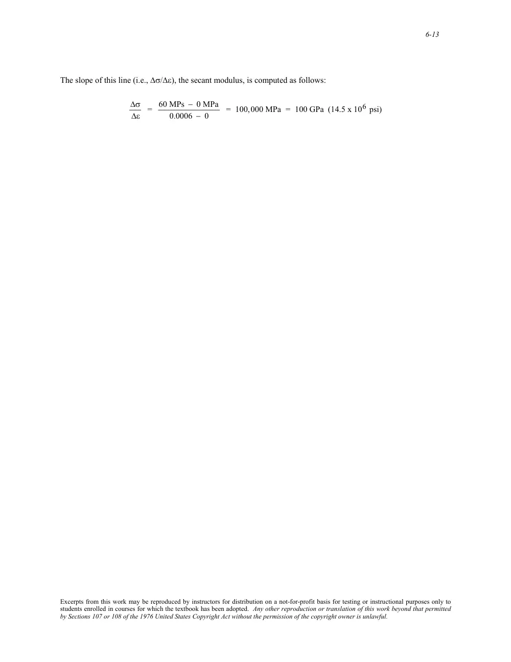6-13 The slope of this line (i.e., ∆σ/∆ε), the secant modulus, is computed as follows: ∆σ ∆ε = 60 MPs − 0 MPa 0.0006 − 0 = 100,000 MPa = 100 GPa (14.5 x 106 psi) Excerpts from this work may be reproduced by instructors for distribution on a not-for-profit basis for testing or instructional purposes only to students enrolled in courses for which the textbook has been adopted. Any other reproduction or translation of this work beyond that permitted by Sections 107 or 108 of the 1976 United States Copyright Act without the permission of the copyright owner is unlawful. 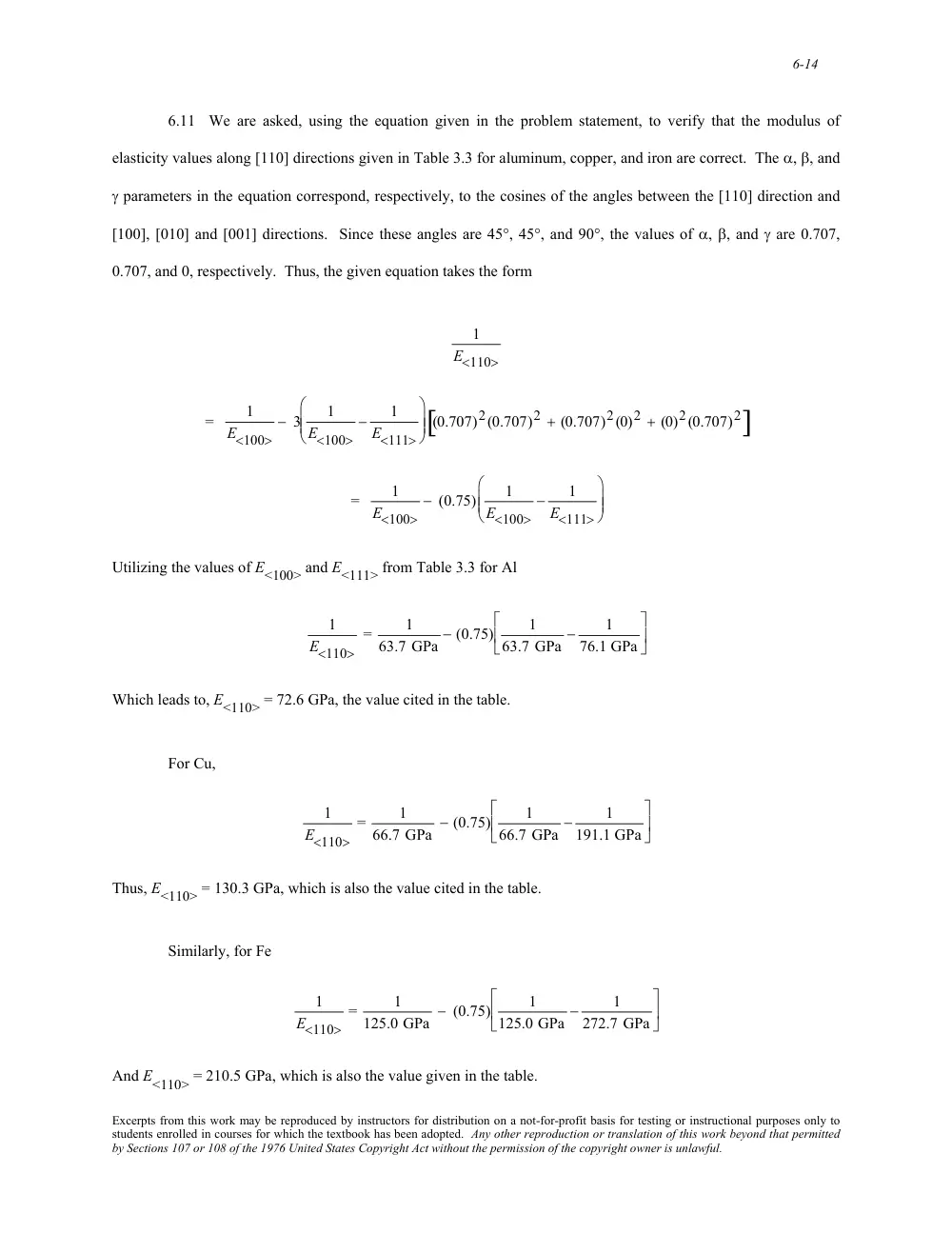6-14 6.11 We are asked, using the equation given in the problem statement, to verify that the modulus of elasticity values along [110] directions given in Table 3.3 for aluminum, copper, and iron are correct. The α, β, and γ parameters in the equation correspond, respectively, to the cosines of the angles between the [110] direction and [100], [010] and [001] directions. Since these angles are 45°, 45°, and 90°, the values of α, β, and γ are 0.707, 0.707, and 0, respectively. Thus, the given equation takes the form 1 E<110> = 1 E<100> − 3 1 E<100> − 1 E<111> ⎛ ⎝ ⎜ ⎜ ⎞ ⎠ ⎟ ⎟ (0.707)2(0.707)2 + (0.707)2(0)2 + (0)2(0.707)2 [ ] = 1 E<100> − (0.75) 1 E<100> − 1 E<111> ⎛ ⎝ ⎜ ⎜ ⎞ ⎠ ⎟ ⎟ Utilizing the values of E<100> and E<111> from Table 3.3 for Al 1 E<110> = 1 63.7 GPa − (0.75) 1 63.7 GPa − 1 76.1 GPa ⎡ ⎣ ⎢ ⎤ ⎦ ⎥ Which leads to, E<110> = 72.6 GPa, the value cited in the table. For Cu, 1 E<110> = 1 66.7 GPa − (0.75) 1 66.7 GPa − 1 191.1 GPa ⎡ ⎣ ⎢ ⎤ ⎦ ⎥ Thus, E<110> = 130.3 GPa, which is also the value cited in the table. Similarly, for Fe 1 E<110> = 1 125.0 GPa − (0.75) 1 125.0 GPa − 1 272.7 GPa ⎡ ⎣ ⎢ ⎤ ⎦ ⎥ And E<110> = 210.5 GPa, which is also the value given in the table. Excerpts from this work may be reproduced by instructors for distribution on a not-for-profit basis for testing or instructional purposes only to students enrolled in courses for which the textbook has been adopted. Any other reproduction or translation of this work beyond that permitted by Sections 107 or 108 of the 1976 United States Copyright Act without the permission of the copyright owner is unlawful. 6-16 6.12 This problem asks that we derive an expression for the dependence of the modulus of elasticity, E, on the parameters A, B, and n in Equation 6.25. It is first necessary to take dEN/dr in order to obtain an expression for the force F; this is accomplished as follows: F = dEN dr = d − A r ⎛ ⎝ ⎜ ⎞ ⎠ ⎟ dr + d B rn ⎛ ⎝ ⎜ ⎞ ⎠ ⎟ dr = A r2 − nB r(n+1) The second step is to set this dEN/dr expression equal to zero and then solve for r (= r0). The algebra for this procedure is carried out in Problem 2.14, with the result that r0 = A nB ⎛ ⎝ ⎜ ⎞ ⎠ ⎟ 1/(1 − n) Next it becomes necessary to take the derivative of the force (dF/dr), which is accomplished as follows: dF dr = d A r2 ⎛ ⎝ ⎜ ⎞ ⎠ ⎟ dr + d − nB r(n+1) ⎛ ⎝ ⎜ ⎞ ⎠ ⎟ dr = − 2A r3 + (n)(n + 1)B r(n+2) Now, substitution of the above expression for r0 into this equation yields dF dr ⎛ ⎝ ⎜ ⎞ ⎠ ⎟ r0 = − 2A A nB ⎛ ⎝ ⎜ ⎞ ⎠ ⎟ 3/(1−n) + (n)(n + 1) B A nB ⎛ ⎝ ⎜ ⎞ ⎠ ⎟ (n+2)/(1−n) which is the expression to which the modulus of elasticity is proportional. Excerpts from this work may be reproduced by instructors for distribution on a not-for-profit basis for testing or instructional purposes only to students enrolled in courses for which the textbook has been adopted. Any other reproduction or translation of this work beyond that permitted by Sections 107 or 108 of the 1976 United States Copyright Act without the permission of the copyright owner is unlawful. 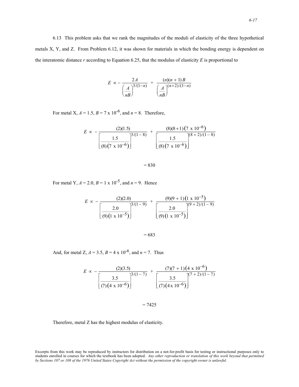6-17 6.13 This problem asks that we rank the magnitudes of the moduli of elasticity of the three hypothetical metals X, Y, and Z. From Problem 6.12, it was shown for materials in which the bonding energy is dependent on the interatomic distance r according to Equation 6.25, that the modulus of elasticity E is proportional to E ∝ − 2A A nB ⎛ ⎝ ⎜ ⎞ ⎠ ⎟ 3/(1−n) + (n)(n + 1) B A nB ⎛ ⎝ ⎜ ⎞ ⎠ ⎟ (n+2)/(1−n) For metal X, A = 1.5, B = 7 x 10-6, and n = 8. Therefore, E ∝ − (2)(1.5) 1.5 (8)(7 x 10−6) ⎡ ⎣ ⎢ ⎢ ⎤ ⎦ ⎥ ⎥ 3/(1 − 8) + (8)(8+1)(7 x 10−6) 1.5 (8)(7 x 10−6) ⎡ ⎣ ⎢ ⎢ ⎤ ⎦ ⎥ ⎥ (8 + 2)/(1 − 8) = 830 For metal Y, A = 2.0, B = 1 x 10-5, and n = 9. Hence E ∝ − (2)(2.0) 2.0 (9)(1 x 10−5) ⎡ ⎣ ⎢ ⎢ ⎤ ⎦ ⎥ ⎥ 3/(1 − 9) + (9)(9 + 1)(1 x 10−5) 2.0 (9)(1 x 10−5) ⎡ ⎣ ⎢ ⎢ ⎤ ⎦ ⎥ ⎥ (9 + 2)/(1 − 9) = 683 And, for metal Z, A = 3.5, B = 4 x 10-6, and n = 7. Thus E ∝ − (2)(3.5) 3.5 (7)(4 x 10−6) ⎡ ⎣ ⎢ ⎢ ⎤ ⎦ ⎥ ⎥ 3/(1 − 7) + (7)(7 + 1)(4 x 10−6) 3.5 (7)(4 x 10−6) ⎡ ⎣ ⎢ ⎢ ⎤ ⎦ ⎥ ⎥ (7 + 2)/(1 − 7) = 7425 Therefore, metal Z has the highest modulus of elasticity. Excerpts from this work may be reproduced by instructors for distribution on a not-for-profit basis for testing or instructional purposes only to students enrolled in courses for which the textbook has been adopted. Any other reproduction or translation of this work beyond that permitted by Sections 107 or 108 of the 1976 United States Copyright Act without the permission of the copyright owner is unlawful. 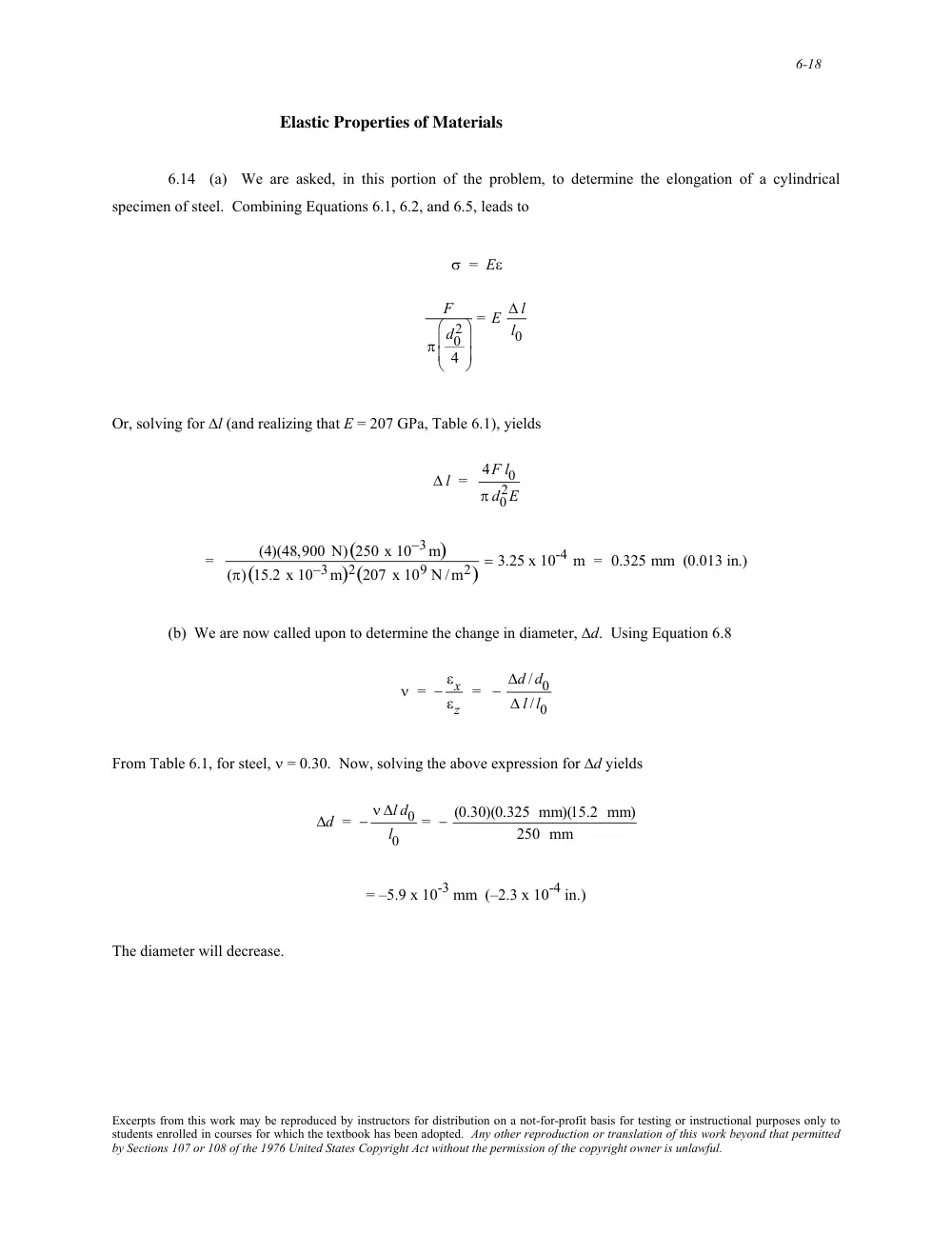6-18 Elastic Properties of Materials 6.14 (a) We are asked, in this portion of the problem, to determine the elongation of a cylindrical specimen of steel. Combining Equations 6.1, 6.2, and 6.5, leads to σ = Eε F π d0 2 4 ⎛ ⎝ ⎜ ⎜ ⎞ ⎠ ⎟ ⎟ = E ∆ l l0 Or, solving for ∆l (and realizing that E = 207 GPa, Table 6.1), yields ∆ l = 4F l0 π d0 2E = (4)(48,900 N)(250 x 10−3m) (π)(15.2 x 10−3m)2(207 x 109 N /m2) = 3.25 x 10-4 m = 0.325 mm (0.013 in.) (b) We are now called upon to determine the change in diameter, ∆d. Using Equation 6.8 ν = − εx εz = − ∆d /d0 ∆ l /l0 From Table 6.1, for steel, ν = 0.30. Now, solving the above expression for ∆d yields ∆d = − ν ∆l d0 l0 = − (0.30)(0.325 mm)(15.2 mm) 250 mm = –5.9 x 10-3 mm (–2.3 x 10-4 in.) The diameter will decrease. Excerpts from this work may be reproduced by instructors for distribution on a not-for-profit basis for testing or instructional purposes only to students enrolled in courses for which the textbook has been adopted. Any other reproduction or translation of this work beyond that permitted by Sections 107 or 108 of the 1976 United States Copyright Act without the permission of the copyright owner is unlawful. 6-19 6.15 This problem asks that we calculate the force necessary to produce a reduction in diameter of 2.5 x 10-3 mm for a cylindrical bar of aluminum. For a cylindrical specimen, the cross-sectional area is equal to A0 = π d0 2 4 Now, combining Equations 6.1 and 6.5 leads to σ = F A0 = F πd0 2 4 = Eεz And, since from Equation 6.8 εz = − εx ν = − ∆d d0 ν = − ∆d νd0 Substitution of this equation into the above expression gives F πd0 2 4 = E − ∆d νd0 ⎛ ⎝ ⎜ ⎜ ⎞ ⎠ ⎟ ⎟ And, solving for F leads to F = − d0∆d π E 4ν From Table 6.1, for aluminum, ν = 0.33 and E = 69 GPa. Thus, F = − (19 x 10−3 m)(−2.5 x 10−6 m)(π)(69 x 109 N /m2) (4)(0.33) = 7,800 N (1785 lbf) Excerpts from this work may be reproduced by instructors for distribution on a not-for-profit basis for testing or instructional purposes only to students enrolled in courses for which the textbook has been adopted. Any other reproduction or translation of this work beyond that permitted by Sections 107 or 108 of the 1976 United States Copyright Act without the permission of the copyright owner is unlawful. 6-20 6.16 This problem asks that we compute Poisson's ratio for the metal alloy. From Equations 6.5 and 6.1 εz = σ E = F A0E = F π d0 2 ⎛ ⎝ ⎜ ⎞ ⎠ ⎟ 2 E = 4F π d0 2 E Since the transverse strain εx is just εx = ∆d d0 and Poisson's ratio is defined by Equation 6.8, then ν = − εx εz = − ∆d /d0 4F π d0 2E ⎛ ⎝ ⎜ ⎜ ⎞ ⎠ ⎟ ⎟ = − d0∆d π E 4F = − (10 x 10−3 m)(−7 x 10−6 m) (π)(100 x 109 N /m2) (4)(15,000 N) = 0.367 Excerpts from this work may be reproduced by instructors for distribution on a not-for-profit basis for testing or instructional purposes only to students enrolled in courses for which the textbook has been adopted. Any other reproduction or translation of this work beyond that permitted by Sections 107 or 108 of the 1976 United States Copyright Act without the permission of the copyright owner is unlawful. 6-21 6.17 This problem asks that we compute the original length of a cylindrical specimen that is stressed in compression. It is first convenient to compute the lateral strain εx as εx = ∆d d0 = 30.04 mm− 30.00 mm 30.00 mm = 1.33 x 10-3 In order to determine the longitudinal strain εz we need Poisson's ratio, which may be computed using Equation 6.9; solving for ν yields ν = E 2G − 1 = 65.5 x 103 MPa (2)(25.4 x 103 MPa) − 1 = 0.289 Now εz may be computed from Equation 6.8 as εz = − εx ν = − 1.33 x 10−3 0.289 = − 4.60 x 10-3 Now solving for l0 using Equation 6.2 l0 = li 1 + εz = 105.20 mm 1 − 4.60 x 10−3 = 105.69 mm Excerpts from this work may be reproduced by instructors for distribution on a not-for-profit basis for testing or instructional purposes only to students enrolled in courses for which the textbook has been adopted. Any other reproduction or translation of this work beyond that permitted by Sections 107 or 108 of the 1976 United States Copyright Act without the permission of the copyright owner is unlawful. 6-22 6.18 This problem asks that we calculate the modulus of elasticity of a metal that is stressed in tension. Combining Equations 6.5 and 6.1 leads to E = σ εz = F A0εz = F εzπ d0 2 ⎛ ⎝ ⎜ ⎞ ⎠ ⎟ 2 = 4F εzπ d0 2 From the definition of Poisson's ratio, (Equation 6.8) and realizing that for the transverse strain, εx= ∆d d0 εz = − εx ν = − ∆d d0ν Therefore, substitution of this expression for εz into the above equation yields E = 4F εzπ d0 2 = 4F ν π d0∆d = (4)(1500 N)(0.35) π(10 × 10−3m)(6.7 × 10−7 m) = 1011 Pa = 100 GPa (14.7 x 106 psi) Excerpts from this work may be reproduced by instructors for distribution on a not-for-profit basis for testing or instructional purposes only to students enrolled in courses for which the textbook has been adopted. Any other reproduction or translation of this work beyond that permitted by Sections 107 or 108 of the 1976 United States Copyright Act without the permission of the copyright owner is unlawful. 6-23 6.19 We are asked to ascertain whether or not it is possible to compute, for brass, the magnitude of the load necessary to produce an elongation of 1.9 mm (0.075 in.). It is first necessary to compute the strain at yielding from the yield strength and the elastic modulus, and then the strain experienced by the test specimen. Then, if ε(test) < ε(yield) deformation is elastic, and the load may be computed using Equations 6.1 and 6.5. However, if ε(test) > ε(yield) computation of the load is not possible inasmuch as deformation is plastic and we have neither a stress-strain plot nor a mathematical expression relating plastic stress and strain. We compute these two strain values as ε(test) = ∆l l0 = 1.9 mm 380 mm = 0.005 and ε(yield) = σ y E = 240 MPa 110 x 103 MPa = 0.0022 Therefore, computation of the load is not possible since ε(test) > ε(yield). Excerpts from this work may be reproduced by instructors for distribution on a not-for-profit basis for testing or instructional purposes only to students enrolled in courses for which the textbook has been adopted. Any other reproduction or translation of this work beyond that permitted by Sections 107 or 108 of the 1976 United States Copyright Act without the permission of the copyright owner is unlawful. 6-2 ∑F x' = 0 which means that PÕ− P cos θ = 0 Or that P' = P cos θ Now it is possible to write an expression for the stress σ' in terms of P' and A' using the above expression and the relationship between A and A' [Figure (a)]: σ' = PÕ AÕ = P cosθ A cosθ = P A cos2θ However, it is the case that P/A = σ; and, after making this substitution into the above expression, we have Equation 6.4a--that is σ' = σ cos2θ Now, for static equilibrium in the y' direction, it is necessary that ∑FyÕ = 0 = −VÕ+ Psinθ Or V' = Psinθ Excerpts from this work may be reproduced by instructors for distribution on a not-for-profit basis for testing or instructional purposes only to students enrolled in courses for which the textbook has been adopted. Any other reproduction or translation of this work beyond that permitted by Sections 107 or 108 of the 1976 United States Copyright Act without the permission of the copyright owner is unlawful. 6-3 We now write an expression for τ' as τÕ= VÕ AÕ And, substitution of the above equation for V' and also the expression for A' gives τ' = VÕ AÕ = Psinθ A cosθ = P A sinθ cosθ = σ sinθ cosθ which is just Equation 6.4b. Excerpts from this work may be reproduced by instructors for distribution on a not-for-profit basis for testing or instructional purposes only to students enrolled in courses for which the textbook has been adopted. Any other reproduction or translation of this work beyond that permitted by Sections 107 or 108 of the 1976 United States Copyright Act without the permission of the copyright owner is unlawful. 6-4 6.2 (a) Below are plotted curves of cos2θ (for σ' ) and sin θ cos θ (for τ') versus θ. (b) The maximum normal stress occurs at an inclination angle of 0°. (c) The maximum shear stress occurs at an inclination angle of 45°. Excerpts from this work may be reproduced by instructors for distribution on a not-for-profit basis for testing or instructional purposes only to students enrolled in courses for which the textbook has been adopted. Any other reproduction or translation of this work beyond that permitted by Sections 107 or 108 of the 1976 United States Copyright Act without the permission of the copyright owner is unlawful. 6-24 6.20 (a) This part of the problem asks that we ascertain which of the metals in Table 6.1 experience an elongation of less than 0.072 mm when subjected to a tensile stress of 50 MPa. The maximum strain that may be sustained, (using Equation 6.2) is just ε = ∆l l0 = 0.072 mm 150 mm = 4.8 x 10-4 Since the stress level is given (50 MPa), using Equation 6.5 it is possible to compute the minimum modulus of elasticity which is required to yield this minimum strain. Hence E = σ ε = 50 MPa 4.8 x 10−4 = 104.2 GPa Which means that those metals with moduli of elasticity greater than this value are acceptable candidates--namely, Cu, Ni, steel, Ti and W. (b) This portion of the problem further stipulates that the maximum permissible diameter decrease is 2.3 x 10-3 mm when the tensile stress of 50 MPa is applied. This translates into a maximum lateral strain εx (max) as εx(max) = ∆d d0 = −2.3 x 10−3 mm 15.0 mm = −1.53 x 10-4 But, since the specimen contracts in this lateral direction, and we are concerned that this strain be less than 1.53 x 10-4, then the criterion for this part of the problem may be stipulated as − ∆d d0 < 1.53 x 10-4. Now, Poisson’s ratio is defined by Equation 6.8 as ν = − εx εz For each of the metal alloys let us consider a possible lateral strain, εx = ∆d d0 . Furthermore, since the deformation is elastic, then, from Equation 6.5, the longitudinal strain, εz is equal to εz = σ E Substituting these expressions for εx and εz into the definition of Poisson’s ratio we have Excerpts from this work may be reproduced by instructors for distribution on a not-for-profit basis for testing or instructional purposes only to students enrolled in courses for which the textbook has been adopted. Any other reproduction or translation of this work beyond that permitted by Sections 107 or 108 of the 1976 United States Copyright Act without the permission of the copyright owner is unlawful. 6-25 ν = − εx εz =− ∆d d0 σ E which leads to the following: − ∆d d0 = νσ E Using values for ν and E found in Table 6.1 for the six metal alloys that satisfy the criterion for part (a), and for σ = 50 MPa, we are able to compute a − ∆d d0 for each alloy as follows: − ∆d d0 (brass) = (0.34)(50 x 106 N /m2) 97 x 109 N /m2 = 1.75 x 10−4 − ∆d d0 (copper) = (0.34)(50 x 106 N /m2) 110 x 109 N /m2 = 1.55 x 10−4 − ∆d d0 (titanium) = (0.34)(50 x 106 N /m2) 107 x 109 N /m2 = 1.59 x 10−4 − ∆d d0 (nickel) = (0.31)(50 x 106 N /m2) 207 x 109 N /m2 = 7.49 x 10−5 − ∆d d0 (steel) = (0.30)(50 x 106 N /m2) 207 x 109 N /m2 = 7.25 x 10−5 − ∆d d0 (tungsten) = (0.28)(50 x 106 N /m2) 407 x 109 N /m2 = 3.44 x 10−5 Thus, the brass, copper, and titanium alloys will experience a negative transverse strain greater than 1.53 x 10-4. This means that the following alloys satisfy the criteria for both parts (a) and (b) of this problem: nickel, steel, and tungsten. Excerpts from this work may be reproduced by instructors for distribution on a not-for-profit basis for testing or instructional purposes only to students enrolled in courses for which the textbook has been adopted. Any other reproduction or translation of this work beyond that permitted by Sections 107 or 108 of the 1976 United States Copyright Act without the permission of the copyright owner is unlawful. 6-26 6.21 (a) This portion of the problem asks that we compute the elongation of the brass specimen. The first calculation necessary is that of the applied stress using Equation 6.1, as σ = F A0 = F π d0 2 ⎛ ⎝ ⎜ ⎞ ⎠ ⎟ 2 = 10,000 N π 10 x 10−3 m 2 ⎛ ⎝ ⎜ ⎜ ⎞ ⎠ ⎟ ⎟ 2 = 127 MPa (17,900 psi) From the stress-strain plot in Figure 6.12, this stress corresponds to a strain of about 1.5 x 10-3. From the definition of strain, Equation 6.2 ∆l = εl0 = (1.5 x 10-3)(101.6 mm) = 0.15 mm (6.0 x 10-3 in.) (b) In order to determine the reduction in diameter ∆d, it is necessary to use Equation 6.8 and the definition of lateral strain (i.e., εx = ∆d/d0) as follows ∆d = d0εx = −d0νεz = −(10 mm)(0.35)(1.5 x 10-3) = –5.25 x 10-3 mm (–2.05 x 10-4 in.) Excerpts from this work may be reproduced by instructors for distribution on a not-for-profit basis for testing or instructional purposes only to students enrolled in courses for which the textbook has been adopted. Any other reproduction or translation of this work beyond that permitted by Sections 107 or 108 of the 1976 United States Copyright Act without the permission of the copyright owner is unlawful. 6-27 6.22 This problem asks that we assess the four alloys relative to the two criteria presented. The first criterion is that the material not experience plastic deformation when the tensile load of 35,000 N is applied; this means that the stress corresponding to this load not exceed the yield strength of the material. Upon computing the stress σ = F A0 = F π d0 2 ⎛ ⎝ ⎜ ⎞ ⎠ ⎟ 2 = 35,000 N π 15 x 10−3 m 2 ⎛ ⎝ ⎜ ⎜ ⎞ ⎠ ⎟ ⎟ 2 = 200 x 106 N/m2 = 200 MPa Of the alloys listed, the Al, Ti and steel alloys have yield strengths greater than 200 MPa. Relative to the second criterion (i.e., that ∆d be less than 1.2 x 10-2 mm), it is necessary to calculate the change in diameter ∆d for these three alloys. From Equation 6.8 ν = − εx εz = − ∆d d0 σ E = − E ∆d σ d0 Now, solving for ∆d from this expression, ∆d = − νσ d0 E For the aluminum alloy ∆d = − (0.33)(200 MPa)(15 mm) 70 x 103MPa = −1.41 x 10-3 mm Therefore, the Al alloy is not a candidate. For the steel alloy ∆d = − (0.27)(200 MPa)(15 mm) 205 x 103MPa = − 0.40 x 10-2 mm Therefore, the steel is a candidate. Excerpts from this work may be reproduced by instructors for distribution on a not-for-profit basis for testing or instructional purposes only to students enrolled in courses for which the textbook has been adopted. Any other reproduction or translation of this work beyond that permitted by Sections 107 or 108 of the 1976 United States Copyright Act without the permission of the copyright owner is unlawful. 6-28 For the Ti alloy ∆d = − (0.36)(200 MPa)(15 mm) 105 x 103 MPa = −1.0 x 10-2 mm Hence, the titanium alloy is also a candidate. Excerpts from this work may be reproduced by instructors for distribution on a not-for-profit basis for testing or instructional purposes only to students enrolled in courses for which the textbook has been adopted. Any other reproduction or translation of this work beyond that permitted by Sections 107 or 108 of the 1976 United States Copyright Act without the permission of the copyright owner is unlawful. 6-29 6.23 This problem asks that we ascertain which of four metal alloys will not (1) experience plastic deformation, and (2) elongate more than 1.3 mm when a tensile load of 29,000 N is applied. It is first necessary to compute the stress using Equation 6.1; a material to be used for this application must necessarily have a yield strength greater than this value. Thus, σ = F A0 = 29,000 N π 12.7 x 10−3 m 2 ⎛ ⎝ ⎜ ⎜ ⎞ ⎠ ⎟ ⎟ 2 = 230 MPa Of the metal alloys listed, aluminum, brass and steel have yield strengths greater than this stress. Next, we must compute the elongation produced in aluminum, brass, and steel using Equations 6.2 and 6.5 in order to determine whether or not this elongation is less than 1.3 mm. For aluminum ∆l = σ l0 E = (230 MPa)(500 mm) 70 x 103 MPa = 1.64 mm Thus, aluminum is not a candidate. For brass ∆l = σ l0 E = (230 MPa)(500 mm) 100 x 103 MPa = 1.15 mm Thus, brass is a candidate. And, for steel ∆l = σ l0 E = (230 MPa)(500 mm) 207 x 103MPa = 0.56 mm Therefore, of these four alloys, only brass and steel satisfy the stipulated criteria. Excerpts from this work may be reproduced by instructors for distribution on a not-for-profit basis for testing or instructional purposes only to students enrolled in courses for which the textbook has been adopted. Any other reproduction or translation of this work beyond that permitted by Sections 107 or 108 of the 1976 United States Copyright Act without the permission of the copyright owner is unlawful. 6-30 Tensile Properties 6.24 Using the stress-strain plot for a steel alloy (Figure 6.21), we are asked to determine several of its mechanical characteristics. (a) The elastic modulus is just the slope of the initial linear portion of the curve; or, from the inset and using Equation 6.10 E = σ2 − σ1 ε2 − ε1 = (1300 − 0) MPa (6.25 x 10−3 − 0) = 210 x 103 MPa = 210 GPa (30.5 x 106 psi) The value given in Table 6.1 is 207 GPa. (b) The proportional limit is the stress level at which linearity of the stress-strain curve ends, which is approximately 1370 MPa (200,000 psi). (c) The 0.002 strain offset line intersects the stress-strain curve at approximately 1570 MPa (228,000 psi). (d) The tensile strength (the maximum on the curve) is approximately 1970 MPa (285,000 psi). Excerpts from this work may be reproduced by instructors for distribution on a not-for-profit basis for testing or instructional purposes only to students enrolled in courses for which the textbook has been adopted. Any other reproduction or translation of this work beyond that permitted by Sections 107 or 108 of the 1976 United States Copyright Act without the permission of the copyright owner is unlawful. 6-31 6.25 We are asked to calculate the radius of a cylindrical brass specimen in order to produce an elongation of 5 mm when a load of 100,000 N is applied. It first becomes necessary to compute the strain corresponding to this elongation using Equation 6.2 as ε = ∆l l0 = 5 mm 100 mm = 5 x 10-2 From Figure 6.12, a stress of 335 MPa (49,000 psi) corresponds to this strain. Since for a cylindrical specimen, stress, force, and initial radius r0 are related as σ = F π r0 2 then r0 = F π σ = 100,000 N π(335 x 106 N /m2) = 0.0097 m = 9.7 mm (0.38 in.) Excerpts from this work may be reproduced by instructors for distribution on a not-for-profit basis for testing or instructional purposes only to students enrolled in courses for which the textbook has been adopted. Any other reproduction or translation of this work beyond that permitted by Sections 107 or 108 of the 1976 United States Copyright Act without the permission of the copyright owner is unlawful. 6-32 6.26 This problem asks us to determine the deformation characteristics of a steel specimen, the stress- strain behavior for which is shown in Figure 6.21. (a) In order to ascertain whether the deformation is elastic or plastic, we must first compute the stress, then locate it on the stress-strain curve, and, finally, note whether this point is on the elastic or plastic region. Thus, from Equation 6.1 σ = F A0 = 140,000 N π 10 x 10−3 m 2 ⎛ ⎝ ⎜ ⎜ ⎞ ⎠ ⎟ ⎟ 2 = 1782 MPa (250,000 psi) The 1782 MPa point is beyond the linear portion of the curve, and, therefore, the deformation will be both elastic and plastic. (b) This portion of the problem asks us to compute the increase in specimen length. From the stress-strain curve, the strain at 1782 MPa is approximately 0.017. Thus, from Equation 6.2 ∆l = εl0 = (0.017)(500 mm) = 8.5 mm (0.34 in.) Excerpts from this work may be reproduced by instructors for distribution on a not-for-profit basis for testing or instructional purposes only to students enrolled in courses for which the textbook has been adopted. Any other reproduction or translation of this work beyond that permitted by Sections 107 or 108 of the 1976 United States Copyright Act without the permission of the copyright owner is unlawful. 6