MECH 340 Lecture, Fall 2007

7-1 CHAPTER 7 DISLOCATIONS AND STRENGTHENING MECHANISMS PROBLEM SOLUTIONS Basic Concepts of Dislocations Characteristics of Dislocations 7.1 The dislocation density is just the total dislocation length per unit volume of material (in this case per cubic millimeters). Thus, the total length in 1000 mm3 of material having a density of 105 mm-2 is just (105 mm-2)(1000 mm3) = 108 mm = 105 m = 62 mi Similarly, for a dislocation density of 109 mm-2, the total length is (109 mm-2)(1000 mm3) = 1012 mm = 109 m = 6.2 x 105 mi Excerpts from this work may be reproduced by instructors for distribution on a not-for-profit basis for testing or instructional purposes only to students enrolled in courses for which the textbook has been adopted. Any other reproduction or translation of this work beyond that permitted by Sections 107 or 108 of the 1976 United States Copyright Act without the permission of the copyright owner is unlawful. 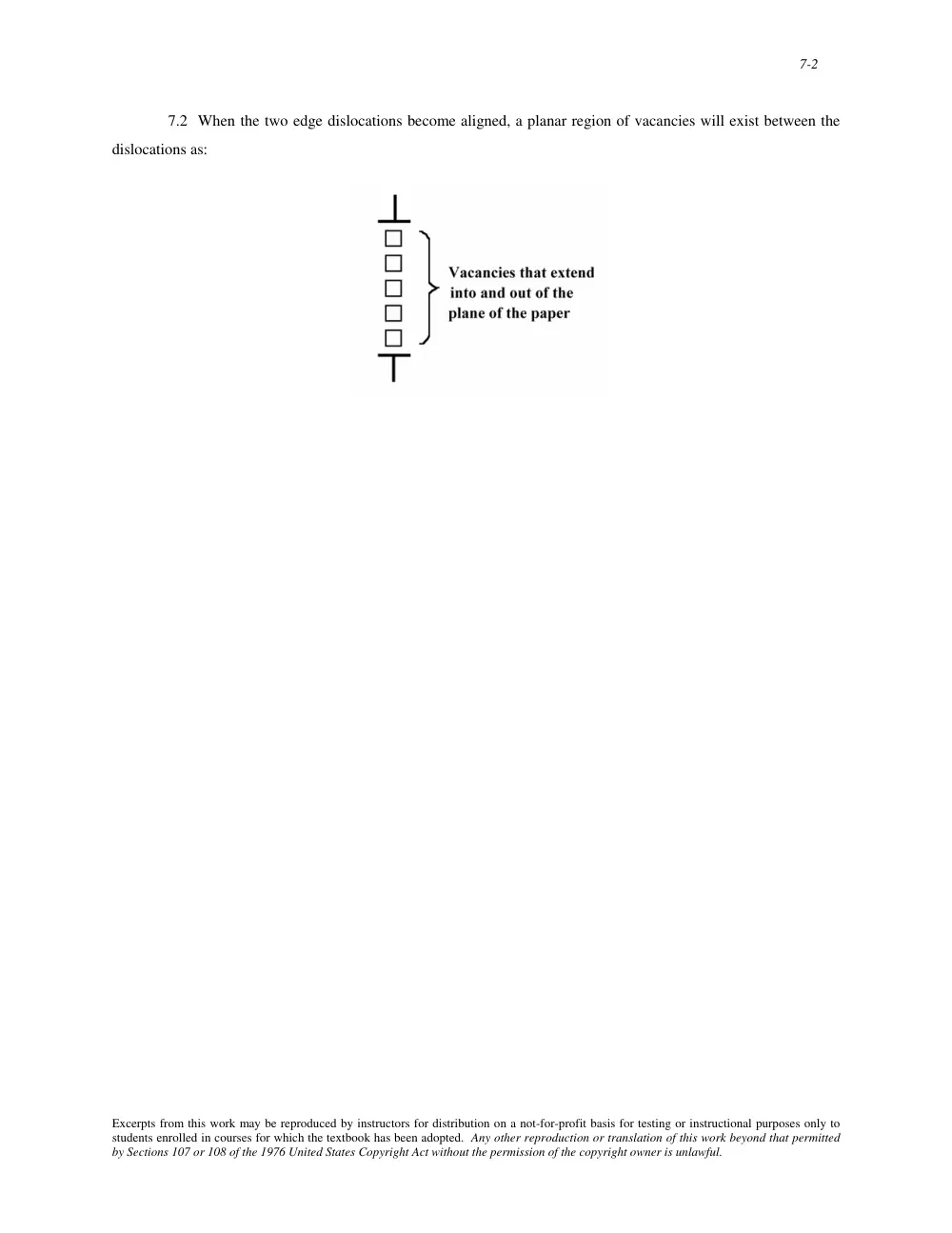7-2 7.2 When the two edge dislocations become aligned, a planar region of vacancies will exist between the dislocations as: Excerpts from this work may be reproduced by instructors for distribution on a not-for-profit basis for testing or instructional purposes only to students enrolled in courses for which the textbook has been adopted. Any other reproduction or translation of this work beyond that permitted by Sections 107 or 108 of the 1976 United States Copyright Act without the permission of the copyright owner is unlawful. 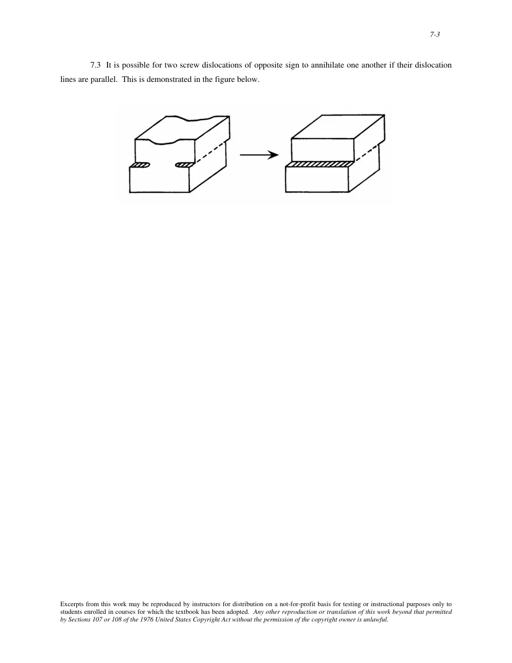7-3 7.3 It is possible for two screw dislocations of opposite sign to annihilate one another if their dislocation lines are parallel. This is demonstrated in the figure below. Excerpts from this work may be reproduced by instructors for distribution on a not-for-profit basis for testing or instructional purposes only to students enrolled in courses for which the textbook has been adopted. Any other reproduction or translation of this work beyond that permitted by Sections 107 or 108 of the 1976 United States Copyright Act without the permission of the copyright owner is unlawful. 7-4 7.4 For the various dislocation types, the relationships between the direction of the applied shear stress and the direction of dislocation line motion are as follows: edge dislocation--parallel screw dislocation--perpendicular mixed dislocation--neither parallel nor perpendicular Excerpts from this work may be reproduced by instructors for distribution on a not-for-profit basis for testing or instructional purposes only to students enrolled in courses for which the textbook has been adopted. Any other reproduction or translation of this work beyond that permitted by Sections 107 or 108 of the 1976 United States Copyright Act without the permission of the copyright owner is unlawful. 7-5 Slip Systems 7.5 (a) A slip system is a crystallographic plane, and, within that plane, a direction along which dislocation motion (or slip) occurs. (b) All metals do not have the same slip system. The reason for this is that for most metals, the slip system will consist of the most densely packed crystallographic plane, and within that plane the most closely packed direction. This plane and direction will vary from crystal structure to crystal structure. Excerpts from this work may be reproduced by instructors for distribution on a not-for-profit basis for testing or instructional purposes only to students enrolled in courses for which the textbook has been adopted. Any other reproduction or translation of this work beyond that permitted by Sections 107 or 108 of the 1976 United States Copyright Act without the permission of the copyright owner is unlawful. 7-9 7.7 Below is shown the atomic packing for a BCC {110}-type plane. The arrows indicate two different <111> type directions. Excerpts from this work may be reproduced by instructors for distribution on a not-for-profit basis for testing or instructional purposes only to students enrolled in courses for which the textbook has been adopted. Any other reproduction or translation of this work beyond that permitted by Sections 107 or 108 of the 1976 United States Copyright Act without the permission of the copyright owner is unlawful. 7-10 7.8 Below is shown the atomic packing for an HCP {0001}-type plane. The arrows indicate three different < 112 0 >-type directions. Excerpts from this work may be reproduced by instructors for distribution on a not-for-profit basis for testing or instructional purposes only to students enrolled in courses for which the textbook has been adopted. Any other reproduction or translation of this work beyond that permitted by Sections 107 or 108 of the 1976 United States Copyright Act without the permission of the copyright owner is unlawful. 7-11 7.9 This problem asks that we compute the magnitudes of the Burgers vectors for copper and iron. For Cu, which has an FCC crystal structure, R = 0.1278 nm (Table 3.1) and a = 2R 2 = 0.3615 nm (Equation 3.1); also, from Equation 7.1a, the Burgers vector for FCC metals is b = a 2 〈110〉 Therefore, the values for u, v, and w in Equation 7.10 are 1, 1, and 0, respectively. Hence, the magnitude of the Burgers vector for Cu is b = a 2 u2 + v2 + w2 = 0.3615 nm 2 (1 )2 + (1 )2 + (0)2 = 0.2556 nm For Fe which has a BCC crystal structure, R = 0.1241 nm (Table 3.1) and a = 4R 3 = 0.2866 nm (Equation 3.3); also, from Equation 7.1b, the Burgers vector for BCC metals is b = a 2 〈111〉 Therefore, the values for u, v, and w in Equation 7.10 are 1, 1, and 1, respectively. Hence, the magnitude of the Burgers vector for Fe is b = 0.2866 nm 2 (1)2 + (1)2 + (1)2 = 0.2482 nm Excerpts from this work may be reproduced by instructors for distribution on a not-for-profit basis for testing or instructional purposes only to students enrolled in courses for which the textbook has been adopted. Any other reproduction or translation of this work beyond that permitted by Sections 107 or 108 of the 1976 United States Copyright Act without the permission of the copyright owner is unlawful. 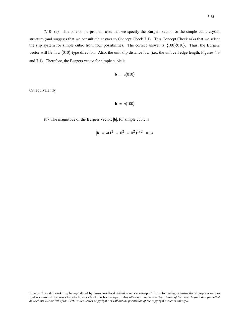7-12 7.10 (a) This part of the problem asks that we specify the Burgers vector for the simple cubic crystal structure (and suggests that we consult the answer to Concept Check 7.1). This Concept Check asks that we select the slip system for simple cubic from four possibilities. The correct answer is 100 { } 010 . Thus, the Burgers vector will lie in a 010 -type direction. Also, the unit slip distance is a (i.e., the unit cell edge length, Figures 4.3 and 7.1). Therefore, the Burgers vector for simple cubic is b = a 010 Or, equivalently b = a 100 (b) The magnitude of the Burgers vector, |b|, for simple cubic is b = a(12 + 02 + 02)1/ 2 = a Excerpts from this work may be reproduced by instructors for distribution on a not-for-profit basis for testing or instructional purposes only to students enrolled in courses for which the textbook has been adopted. Any other reproduction or translation of this work beyond that permitted by Sections 107 or 108 of the 1976 United States Copyright Act without the permission of the copyright owner is unlawful. 7-13 Slip in Single Crystals 7.11 We are asked to compute the Schmid factor for an FCC crystal oriented with its [120] direction parallel to the loading axis. With this scheme, slip may occur on the (111) plane and in the [011 ] direction as noted in the figure below. The angle between the [120] and [011 ] directions, λ, may be determined using Equation 7.6 λ = cos−1 u1u2 + v1v2 + w1w2 u1 2 + v1 2 + w1 2 ( )u2 2 + v2 2 + w2 2 ( ) ⎡ ⎣ ⎢ ⎢ ⎢ ⎤ ⎦ ⎥ ⎥ ⎥ where (for [120]) u1 = 1, v1 = 2, w1 = 0, and (for [011 ]) u2 = 0, v2 = 1, w2 = -1. Therefore, λ is equal to λ = cos−1 (1)(0) + (2)(1) + (0)(−1) [(1)2 + (2)2 + (0)2 ] (0)2 + (1)2 + (−1)2 [ ] ⎡ ⎣ ⎢ ⎢ ⎢ ⎤ ⎦ ⎥ ⎥ ⎥ = cos−1 2 10 ⎛ ⎝ ⎜ ⎜ ⎞ ⎠ ⎟ ⎟ = 50.8° Excerpts from this work may be reproduced by instructors for distribution on a not-for-profit basis for testing or instructional purposes only to students enrolled in courses for which the textbook has been adopted. Any other reproduction or translation of this work beyond that permitted by Sections 107 or 108 of the 1976 United States Copyright Act without the permission of the copyright owner is unlawful. 7-14 Now, the angle φ is equal to the angle between the normal to the (111) plane (which is the [111] direction), and the [120] direction. Again from Equation 7.6, and for u1 = 1, v1 = 1, w1 = 1, u2 = 1, v2 = 2, and w2 = 0, we have φ = cos−1 (1)(1) + (1)(2) + (1)(0) [(1)2 + (1)2 + (1)2 ] (1)2 + (2)2 + (0)2 [ ] ⎡ ⎣ ⎢ ⎢ ⎢ ⎤ ⎦ ⎥ ⎥ ⎥ = cos−1 3 15 ⎛ ⎝ ⎜ ⎜ ⎞ ⎠ ⎟ ⎟ = 39.2° Therefore, the Schmid factor is equal to cos λ cos φ = cos(50.8°) cos(39.2°) = 2 10 ⎛ ⎝ ⎜ ⎜ ⎞ ⎠ ⎟ ⎟ 3 15 ⎛ ⎝ ⎜ ⎞ ⎠ ⎟ = 0.490 Excerpts from this work may be reproduced by instructors for distribution on a not-for-profit basis for testing or instructional purposes only to students enrolled in courses for which the textbook has been adopted. Any other reproduction or translation of this work beyond that permitted by Sections 107 or 108 of the 1976 United States Copyright Act without the permission of the copyright owner is unlawful. 7-15 7.12 This problem calls for us to determine whether or not a metal single crystal having a specific orientation and of given critical resolved shear stress will yield. We are given that φ = 60°, λ = 35°, and that the values of the critical resolved shear stress and applied tensile stress are 6.2 MPa (900 psi) and 12 MPa (1750 psi), respectively. From Equation 7.2 τR = σ cos φ cos λ = (12 MPa)(cos 60°)(cos 35°) = 4.91 MPa (717 psi) Since the resolved shear stress (4.91 MPa) is less that the critical resolved shear stress (6.2 MPa), the single crystal will not yield. However, from Equation 7.4, the stress at which yielding occurs is σ y = τcrss cos φ cos λ = 6.2 MPa (cos 60°)(cos 35°) = 15.1 MPa (2200 psi) Excerpts from this work may be reproduced by instructors for distribution on a not-for-profit basis for testing or instructional purposes only to students enrolled in courses for which the textbook has been adopted. Any other reproduction or translation of this work beyond that permitted by Sections 107 or 108 of the 1976 United States Copyright Act without the permission of the copyright owner is unlawful. 7-16 7.13 We are asked to compute the critical resolved shear stress for Zn. As stipulated in the problem, φ = 65°, while possible values for λ are 30°, 48°, and 78°. (a) Slip will occur along that direction for which (cos φ cos λ) is a maximum, or, in this case, for the largest cos λ. Cosines for the possible λ values are given below. cos(30°) = 0.87 cos(48°) = 0.67 cos(78°) = 0.21 Thus, the slip direction is at an angle of 30° with the tensile axis. (b) From Equation 7.4, the critical resolved shear stress is just τcrss = σ y (cos φ cos λ)max = (2.5 MPa) cos(65°) cos(30°) [ ] = 0.90 MPa (130 psi) Excerpts from this work may be reproduced by instructors for distribution on a not-for-profit basis for testing or instructional purposes only to students enrolled in courses for which the textbook has been adopted. Any other reproduction or translation of this work beyond that permitted by Sections 107 or 108 of the 1976 United States Copyright Act without the permission of the copyright owner is unlawful. 7-17 7.14 This problem asks that we compute the critical resolved shear stress for nickel. In order to do this, we must employ Equation 7.4, but first it is necessary to solve for the angles λ and φ which are shown in the sketch below. The angle λ is the angle between the tensile axis—i.e., along the [001] direction—and the slip direction—i.e., [1 01]. The angle λ may be determined using Equation 7.6 as λ = cos−1 u1u2 + v1v2 + w1w2 u1 2 + v1 2 + w1 2 ( )u2 2 + v2 2 + w2 2 ( ) ⎡ ⎣ ⎢ ⎢ ⎢ ⎤ ⎦ ⎥ ⎥ ⎥ where (for [001]) u1 = 0, v1 = 0, w1 = 1, and (for [1 01]) u2 = –1, v2 = 0, w2 = 1. Therefore, λ is equal to λ = cos−1 (0)(−1) + (0)(0) + (1)(1) [(0)2 + (0)2 + (1)2 ] (−1)2 + (0)2 + (1)2 [ ] ⎡ ⎣ ⎢ ⎢ ⎢ ⎤ ⎦ ⎥ ⎥ ⎥ = cos−1 1 2 ⎛ ⎝ ⎜ ⎜ ⎞ ⎠ ⎟ ⎟ = 45° Furthermore, φ is the angle between the tensile axis—the [001] direction—and the normal to the slip plane—i.e., the (111) plane; for this case this normal is along a [111] direction. Therefore, again using Equation 7.6 Excerpts from this work may be reproduced by instructors for distribution on a not-for-profit basis for testing or instructional purposes only to students enrolled in courses for which the textbook has been adopted. Any other reproduction or translation of this work beyond that permitted by Sections 107 or 108 of the 1976 United States Copyright Act without the permission of the copyright owner is unlawful. 7-18 φ = cos−1 (0)(1) + (0)(1) + (1)(1) [(0)2 + (0)2 + (1)2 ] (1)2 + (1)2 + (1)2 [ ] ⎡ ⎣ ⎢ ⎢ ⎢ ⎤ ⎦ ⎥ ⎥ ⎥ = cos−1 1 3 ⎛ ⎝ ⎜ ⎜ ⎞ ⎠ ⎟ ⎟ = 54.7° And, finally, using Equation 7.4, the critical resolved shear stress is equal to τcrss = σ y (cos φ cos λ) = (13.9 MPa) cos(54.7°) cos(45°) [ ] = (13.9 MPa) 1 3 ⎛ ⎝ ⎜ ⎜ ⎞ ⎠ ⎟ ⎟ 1 2 ⎛ ⎝ ⎜ ⎜ ⎞ ⎠ ⎟ ⎟ = 5.68 MPa (825 psi) Excerpts from this work may be reproduced by instructors for distribution on a not-for-profit basis for testing or instructional purposes only to students enrolled in courses for which the textbook has been adopted. Any other reproduction or translation of this work beyond that permitted by Sections 107 or 108 of the 1976 United States Copyright Act without the permission of the copyright owner is unlawful. 7-19 7.15 This problem asks that, for a metal that has the FCC crystal structure, we compute the applied stress(s) that are required to cause slip to occur on a (111) plane in each of the [11 0], [101 ], and [01 1] directions. In order to solve this problem it is necessary to employ Equation 7.4, but first we need to solve for the for λ and φ angles for the three slip systems. For each of these three slip systems, the φ will be the same—i.e., the angle between the direction of the applied stress, [100] and the normal to the (111) plane, that is, the [111] direction. The angle φ may be determined using Equation 7.6 as φ = cos−1 u1u2 + v1v2 + w1w2 u1 2 + v1 2 + w1 2 ( )u2 2 + v2 2 + w2 2 ( ) ⎡ ⎣ ⎢ ⎢ ⎢ ⎤ ⎦ ⎥ ⎥ ⎥ where (for [100]) u1 = 1, v1 = 0, w1 = 0, and (for [111]) u2 = 1, v2 = 1, w2 = 1. Therefore, φ is equal to φ = cos−1 (1)(1) + (0)(1) + (0)(1) [(1)2 + (0)2 + (0)2 ] (1)2 + (1)2 + (1)2 [ ] ⎡ ⎣ ⎢ ⎢ ⎢ ⎤ ⎦ ⎥ ⎥ ⎥ = cos−1 1 3 ⎛ ⎝ ⎜ ⎜ ⎞ ⎠ ⎟ ⎟ = 54.7° Let us now determine λ for the [11 0] slip direction. Again, using Equation 7.6 where u1 = 1, v1 = 0, w1 = 0 (for [100]), and u2 = 1, v2 = –1, w2 = 0 (for [11 0]. Therefore, λ is determined as λ[100]−[11 0] = cos−1 (1)(1) + (0)(−1) + (0)(0) [(1)2 + (0)2 + (0)2 ] (1)2 + (−1)2 + (0)2 [ ] ⎡ ⎣ ⎢ ⎢ ⎢ ⎤ ⎦ ⎥ ⎥ ⎥ = cos−1 1 2 ⎛ ⎝ ⎜ ⎜ ⎞ ⎠ ⎟ ⎟ = 45° Now, we solve for the yield strength for this (111)– [11 0] slip system using Equation 7.4 as σ y = τcrss (cosφ cos λ) Excerpts from this work may be reproduced by instructors for distribution on a not-for-profit basis for testing or instructional purposes only to students enrolled in courses for which the textbook has been adopted. Any other reproduction or translation of this work beyond that permitted by Sections 107 or 108 of the 1976 United States Copyright Act without the permission of the copyright owner is unlawful. 7-20 = 0.5 MPa cos (54.7°) cos (45°) = 0.5 MPa (0.578) (0.707) = 1.22 MPa Now, we must determine the value of λ for the (111)– [101 ] slip system—that is, the angle between the [100] and [101 ] directions. Again using Equation 7.6 λ[100]−[101 ] = cos−1 (1)(1) + (0)(0) + (0)(−1) [(1)2 + (0)2 + (0)2 ] (1)2 + (0)2 + (−1)2 [ ] ⎡ ⎣ ⎢ ⎢ ⎢ ⎤ ⎦ ⎥ ⎥ ⎥ = cos−1 1 2 ⎛ ⎝ ⎜ ⎜ ⎞ ⎠ ⎟ ⎟ = 45° Thus, since the values of φ and λ for this (111)– [101 ] slip system are the same as for (111)– [11 0], so also will σy be the same—viz 1.22 MPa. And, finally, for the (111)– [01 1] slip system, λ is computed using Equation 7.6 as follows: λ[100]−[01 1] = cos−1 (1)(0) + (0)(−1) + (0)(1) [(1)2 + (0)2 + (0)2 ] (0)2 + (−1)2 + (1)2 [ ] ⎡ ⎣ ⎢ ⎢ ⎢ ⎤ ⎦ ⎥ ⎥ ⎥ = cos−1 (0) = 90° Thus, from Equation 7.4, the yield strength for this slip system is σ y = τcrss (cosφ cos λ) = 0.5 MPa cos (54.7°) cos (90°) = 0.5 MPa (0.578) (0) = ∞ which means that slip will not occur on this (111)– [01 1] slip system. Excerpts from this work may be reproduced by instructors for distribution on a not-for-profit basis for testing or instructional purposes only to students enrolled in courses for which the textbook has been adopted. Any other reproduction or translation of this work beyond that permitted by Sections 107 or 108 of the 1976 United States Copyright Act without the permission of the copyright owner is unlawful. 7-21 7.16 (a) This part of the problem asks, for a BCC metal, that we compute the resolved shear stress in the [11 1] direction on each of the (110), (011), and (101 ) planes. In order to solve this problem it is necessary to employ Equation 7.2, which means that we first need to solve for the for angles λ and φ for the three slip systems. For each of these three slip systems, the λ will be the same—i.e., the angle between the direction of the applied stress, [100] and the slip direction, [11 1]. This angle λ may be determined using Equation 7.6 λ = cos−1 u1u2 + v1v2 + w1w2 u1 2 + v1 2 + w1 2 ( )u2 2 + v2 2 + w2 2 ( ) ⎡ ⎣ ⎢ ⎢ ⎢ ⎤ ⎦ ⎥ ⎥ ⎥ where (for [100]) u1 = 1, v1 = 0, w1 = 0, and (for [11 1]) u2 = 1, v2 = –1, w2 = 1. Therefore, λ is determined as λ = cos−1 (1)(1) + (0)(−1) + (0)(1) [(1)2 + (0)2 + (0)2 ] (1)2 + (−1)2 + (1)2 [ ] ⎡ ⎣ ⎢ ⎢ ⎢ ⎤ ⎦ ⎥ ⎥ ⎥ = cos−1 1 3 ⎛ ⎝ ⎜ ⎜ ⎞ ⎠ ⎟ ⎟ = 54.7° Let us now determine φ for the angle between the direction of the applied tensile stress—i.e., the [100] direction— and the normal to the (110) slip plane—i.e., the [110] direction. Again, using Equation 7.6 where u1 = 1, v1 = 0, w1 = 0 (for [100]), and u2 = 1, v2 = 1, w2 = 0 (for [110]), φ is equal to φ[100]−[110] = cos−1 (1)(1) + (0)(1) + (0)(0) [(1)2 + (0)2 + (0)2 ] (1)2 + (1)2 + (0)2 [ ] ⎡ ⎣ ⎢ ⎢ ⎢ ⎤ ⎦ ⎥ ⎥ ⎥ = cos−1 1 2 ⎛ ⎝ ⎜ ⎜ ⎞ ⎠ ⎟ ⎟ = 45° Now, using Equation 7.2 τR = σ cosφ cos λ we solve for the resolved shear stress for this slip system as Excerpts from this work may be reproduced by instructors for distribution on a not-for-profit basis for testing or instructional purposes only to students enrolled in courses for which the textbook has been adopted. Any other reproduction or translation of this work beyond that permitted by Sections 107 or 108 of the 1976 United States Copyright Act without the permission of the copyright owner is unlawful. 7-22 τR(110)−[11 1] = (4.0 MPa) cos (45°) cos (54.7°) [ ] = (4.0 MPa) (0.707)(0.578) = 1.63 MPa Now, we must determine the value of φ for the (011)– [11 1] slip system—that is, the angle between the direction of the applied stress, [100], and the normal to the (011) plane—i.e., the [011] direction. Again using Equation 7.6 λ[100]−[011] = cos−1 (1)(0) + (0)(1) + (0)(1) [(1)2 + (0)2 + (0)2 ] (0)2 + (1)2 + (1)2 [ ] ⎡ ⎣ ⎢ ⎢ ⎢ ⎤ ⎦ ⎥ ⎥ ⎥ = cos−1 (0) = 90° Thus, the resolved shear stress for this (011)– [11 1] slip system is τR(011)−[11 1] = = (4.0 MPa) cos (90°) cos (54.7°) [ ] = (4.0 MPa) (0)(0.578) = 0 MPa And, finally, it is necessary to determine the value of φ for the (101 )– [11 1] slip system —that is, the angle between the direction of the applied stress, [100], and the normal to the (101 ) plane—i.e., the [101 ] direction. Again using Equation 7.6 λ[100]−[101 ] = cos−1 (1)(1) + (0)(0) + (0)(−1) [(1)2 + (0)2 + (0)2 ] (1)2 + (0)2 + (−1)2 [ ] ⎡ ⎣ ⎢ ⎢ ⎢ ⎤ ⎦ ⎥ ⎥ ⎥ = cos−1 1 2 ⎛ ⎝ ⎜ ⎜ ⎞ ⎠ ⎟ ⎟ = 45° Here, as with the (110)– [11 1] slip system above, the value of φ is 45°, which again leads to τR(101 )−[11 1] = (4.0 MPa) cos (45°) cos(54.7°) [ ] = (4.0 MPa) (0.707)(0.578) = 1.63 MPa (b) The most favored slip system(s) is (are) the one(s) that has (have) the largest τR value. Both (110)– [11 1] and (101 ) −[11 1] slip systems are most favored since they have the same τR (1.63 MPa), which is greater than the τR value for (011) −[11 1] (viz., 0 MPa). Excerpts from this work may be reproduced by instructors for distribution on a not-for-profit basis for testing or instructional purposes only to students enrolled in courses for which the textbook has been adopted. Any other reproduction or translation of this work beyond that permitted by Sections 107 or 108 of the 1976 United States Copyright Act without the permission of the copyright owner is unlawful. 7-23 7.17 This problem asks for us to determine the tensile stress at which a BCC metal yields when the stress is applied along a [121] direction such that slip occurs on a (101) plane and in a [1 11] direction; the critical resolved shear stress for this metal is 2.4 MPa. To solve this problem we use Equation 7.4; however it is first necessary to determine the values of φ and λ. These determinations are possible using Equation 7.6. Now, λ is the angle between [121] and [1 11] directions. Therefore, relative to Equation 7.6 let us take u1 = 1, v1 = 2, and w1 = 1, as well as u2 = –1, v2 = 1, and w2 = 1. This leads to λ = cos−1 u1u2 + v1v2 + w1w2 u1 2 + v1 2 + w1 2 ( )u2 2 + v2 2 + w2 2 ( ) ⎡ ⎣ ⎢ ⎢ ⎢ ⎤ ⎦ ⎥ ⎥ ⎥ = cos−1 (1)(−1) + (2)(1) + (1)(1) [(1)2 + (2)2 + (1)2 ] (−1)2 + (1)2 + (1)2 [ ] ⎧ ⎨ ⎪ ⎩ ⎪ ⎫ ⎬ ⎪ ⎭ ⎪ = cos−1 2 18 ⎛ ⎝ ⎜ ⎜ ⎞ ⎠ ⎟ ⎟ = 61.9° Now for the determination of φ, the normal to the (101) slip plane is the [101] direction. Again using Equation 7.6, where we now take u1 = 1, v1 = 2, w1 = 1 (for [121]), and u2 = 1, v2 = 0, w2 = 1 (for [101]). Thus, φ = cos−1 (1)(1) + (2)(0) + (1)(1) [(1)2 + (2)2 + (1)2 ] (1)2 + (0)2 + (1)2 [ ] ⎧ ⎨ ⎪ ⎩ ⎪ ⎫ ⎬ ⎪ ⎭ ⎪ = cos−1 2 12 ⎛ ⎝ ⎜ ⎜ ⎞ ⎠ ⎟ ⎟ = 54.7° It is now possible to compute the yield stress (using Equation 7.4) as σ y = τcrss cosφ cos λ = 2.4 MPa 2 12 ⎛ ⎝ ⎜ ⎜ ⎞ ⎠ ⎟ ⎟ 2 18 ⎛ ⎝ ⎜ ⎜ ⎞ ⎠ ⎟ ⎟ = 8.82 MPa Excerpts from this work may be reproduced by instructors for distribution on a not-for-profit basis for testing or instructional purposes only to students enrolled in courses for which the textbook has been adopted. Any other reproduction or translation of this work beyond that permitted by Sections 107 or 108 of the 1976 United States Copyright Act without the permission of the copyright owner is unlawful. 7-24 7.18 In order to determine the maximum possible yield strength for a single crystal of Cu pulled in tension, we simply employ Equation 7.5 as σ y = 2τcrss = (2)(0.48 MPa) = 0.96 MPa (140 psi) Excerpts from this work may be reproduced by instructors for distribution on a not-for-profit basis for testing or instructional purposes only to students enrolled in courses for which the textbook has been adopted. Any other reproduction or translation of this work beyond that permitted by Sections 107 or 108 of the 1976 United States Copyright Act without the permission of the copyright owner is unlawful. 7-25 Deformation by Twinning 7.19 Four major differences between deformation by twinning and deformation by slip are as follows: (1) with slip deformation there is no crystallographic reorientation, whereas with twinning there is a reorientation; (2) for slip, the atomic displacements occur in atomic spacing multiples, whereas for twinning, these displacements may be other than by atomic spacing multiples; (3) slip occurs in metals having many slip systems, whereas twinning occurs in metals having relatively few slip systems; and (4) normally slip results in relatively large deformations, whereas only small deformations result for twinning. Excerpts from this work may be reproduced by instructors for distribution on a not-for-profit basis for testing or instructional purposes only to students enrolled in courses for which the textbook has been adopted. Any other reproduction or translation of this work beyond that permitted by Sections 107 or 108 of the 1976 United States Copyright Act without the permission of the copyright owner is unlawful. 7-26 Strengthening by Grain Size Reduction 7.20 Small-angle grain boundaries are not as effective in interfering with the slip process as are high-angle grain boundaries because there is not as much crystallographic misalignment in the grain boundary region for small- angle, and therefore not as much change in slip direction. Excerpts from this work may be reproduced by instructors for distribution on a not-for-profit basis for testing or instructional purposes only to students enrolled in courses for which the textbook has been adopted. Any other reproduction or translation of this work beyond that permitted by Sections 107 or 108 of the 1976 United States Copyright Act without the permission of the copyright owner is unlawful. 7-27 7.21 Hexagonal close packed metals are typically more brittle than FCC and BCC metals because there are fewer slip systems in HCP. Excerpts from this work may be reproduced by instructors for distribution on a not-for-profit basis for testing or instructional purposes only to students enrolled in courses for which the textbook has been adopted. Any other reproduction or translation of this work beyond that permitted by Sections 107 or 108 of the 1976 United States Copyright Act without the permission of the copyright owner is unlawful. 7-28 7.22 These three strengthening mechanisms are described in Sections 7.8, 7.9, and 7.10. Excerpts from this work may be reproduced by instructors for distribution on a not-for-profit basis for testing or instructional purposes only to students enrolled in courses for which the textbook has been adopted. Any other reproduction or translation of this work beyond that permitted by Sections 107 or 108 of the 1976 United States Copyright Act without the permission of the copyright owner is unlawful. 7-29 7.23 (a) Perhaps the easiest way to solve for σ0 and ky in Equation 7.7 is to pick two values each of σy and d-1/2 from Figure 7.15, and then solve two simultaneous equations, which may be set up. For example d-1/2 (mm) -1/2 σy (MPa) 4 75 12 175 The two equations are thus 75 = σ0 + 4k y 175 = σ0 + 12 k y Solution of these equations yield the values of k y = 12.5 MPa (mm)1/2 1810 psi(mm)1/2 [ ] σ0 = 25 MPa (3630 psi) (b) When d = 2.0 x 10-3 mm, d-1/2 = 22.4 mm-1/2, and, using Equation 7.7, σ y = σ0 + k yd-1/2 = (25 MPa) + 12.5 MPa (mm) 1/2 ⎡ ⎣ ⎢ ⎤ ⎦ ⎥ (22.4 mm-1/2) = 305 MPa (44,200 psi) Excerpts from this work may be reproduced by instructors for distribution on a not-for-profit basis for testing or instructional purposes only to students enrolled in courses for which the textbook has been adopted. Any other reproduction or translation of this work beyond that permitted by Sections 107 or 108 of the 1976 United States Copyright Act without the permission of the copyright owner is unlawful. 7-30 7.24 We are asked to determine the grain diameter for an iron which will give a yield strength of 310 MPa (45,000 psi). The best way to solve this problem is to first establish two simultaneous expressions of Equation 7.7, solve for σ0 and ky, and finally determine the value of d when σy = 310 MPa. The data pertaining to this problem may be tabulated as follows: σy d (mm) d-1/2 (mm)-1/2 230 MPa 1 x 10-2 10.0 275 MPa 6 x 10-3 12.91 The two equations thus become 230 MPa = σ0 + (10.0) k y 275 MPa = σ0 + (12.91) k y Which yield the values, σ0 = 75.4 MPa and ky = 15.46 MPa(mm)1/2. At a yield strength of 310 MPa 310 MPa = 75.4 MPa + 15.46 MPa (mm)1/2 [ ]d-1/2 or d-1/2 = 15.17 (mm)-1/2, which gives d = 4.34 x 10-3 mm. Excerpts from this work may be reproduced by instructors for distribution on a not-for-profit basis for testing or instructional purposes only to students enrolled in courses for which the textbook has been adopted. Any other reproduction or translation of this work beyond that permitted by Sections 107 or 108 of the 1976 United States Copyright Act without the permission of the copyright owner is unlawful. 7-31 7.25 This problem asks that we determine the grain size of the brass for which is the subject of Figure 7.19. From Figure 7.19(a), the yield strength of brass at 0%CW is approximately 175 MPa (26,000 psi). This yield strength from Figure 7.15 corresponds to a d-1/2 value of approximately 12.0 (mm)-1/2. Thus, d = 6.9 x 10-3 mm. Excerpts from this work may be reproduced by instructors for distribution on a not-for-profit basis for testing or instructional purposes only to students enrolled in courses for which the textbook has been adopted. Any other reproduction or translation of this work beyond that permitted by Sections 107 or 108 of the 1976 United States Copyright Act without the permission of the copyright owner is unlawful. 7-32 Solid-Solution Strengthening 7.26 Below is shown an edge dislocation and where an interstitial impurity atom would be located. Compressive lattice strains are introduced by the impurity atom. There will be a net reduction in lattice strain energy when these lattice strains partially cancel tensile strains associated with the edge dislocation; such tensile strains exist just below the bottom of the extra half-plane of atoms (Figure 7.4). Excerpts from this work may be reproduced by instructors for distribution on a not-for-profit basis for testing or instructional purposes only to students enrolled in courses for which the textbook has been adopted. Any other reproduction or translation of this work beyond that permitted by Sections 107 or 108 of the 1976 United States Copyright Act without the permission of the copyright owner is unlawful. 7-33 Strain Hardening 7.27 (a) We are asked to show, for a tensile test, that %CW = ε ε + 1 ⎛ ⎝ ⎜ ⎞ ⎠ ⎟ x 100 From Equation 7.8 %CW = A0 − Ad A0 ⎡ ⎣ ⎢ ⎢ ⎤ ⎦ ⎥ ⎥ x 100 = 1 − Ad A0 ⎡ ⎣ ⎢ ⎢ ⎤ ⎦ ⎥ ⎥ x 100 Which is also equal to 1 − l0 ld ⎡ ⎣ ⎢ ⎢ ⎤ ⎦ ⎥ ⎥ x 100 since Ad/A0 = l0/ld, the conservation of volume stipulation given in the problem statement. Now, from the definition of engineering strain (Equation 6.2) ε = ld − l0 l0 = ld l0 −1 Or, l0 ld = 1 ε + 1 Substitution for l0/ ld into the