MECH 340 Lecture, Fall 2008

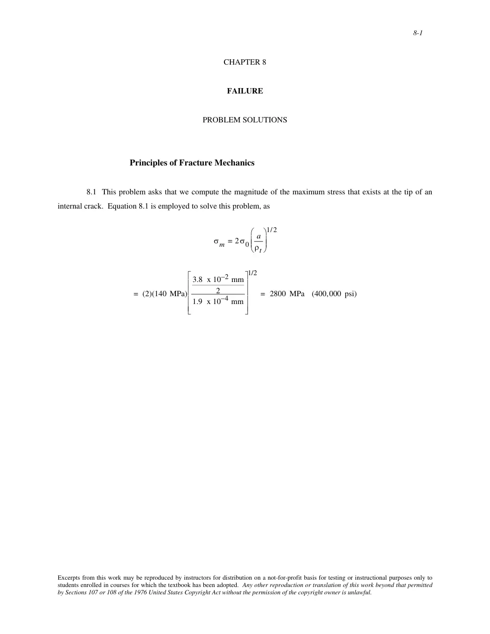
8-1 CHAPTER 8 FAILURE PROBLEM SOLUTIONS Principles of Fracture Mechanics 8.1 This problem asks that we compute the magnitude of the maximum stress that exists at the tip of an internal crack. Equation 8.1 is employed to solve this problem, as σm = 2σ0 a ρt ⎛ ⎝ ⎜ ⎜ ⎞ ⎠ ⎟ ⎟ 1/2 = (2)(140 MPa) 3.8 x 10−2 mm 2 1.9 x 10−4 mm ⎡ ⎣ ⎢ ⎢ ⎢ ⎢ ⎤ ⎦ ⎥ ⎥ ⎥ ⎥ 1/2 = 2800 MPa (400,000 psi) Excerpts from this work may be reproduced by instructors for distribution on a not-for-profit basis for testing or instructional purposes only to students enrolled in courses for which the textbook has been adopted. Any other reproduction or translation of this work beyond that permitted by Sections 107 or 108 of the 1976 United States Copyright Act without the permission of the copyright owner is unlawful. 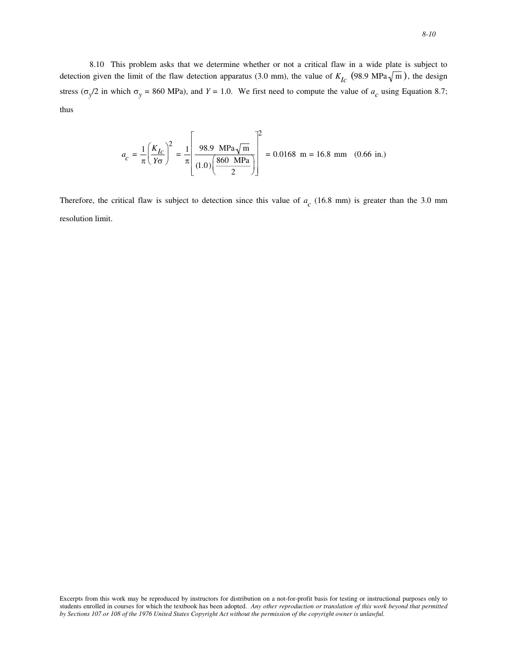8-10 8.10 This problem asks that we determine whether or not a critical flaw in a wide plate is subject to detection given the limit of the flaw detection apparatus (3.0 mm), the value of KIc (98.9 MPa m), the design stress (σy/2 in which σy = 860 MPa), and Y = 1.0. We first need to compute the value of ac using Equation 8.7; thus ac = 1 π KIc Yσ ⎛ ⎝ ⎜ ⎞ ⎠ ⎟ 2 = 1 π 98.9 MPa m (1.0) 860 MPa 2 ⎛ ⎝ ⎜ ⎞ ⎠ ⎟ ⎡ ⎣ ⎢ ⎢ ⎢ ⎢ ⎤ ⎦ ⎥ ⎥ ⎥ ⎥ 2 = 0.0168 m = 16.8 mm (0.66 in.) Therefore, the critical flaw is subject to detection since this value of ac (16.8 mm) is greater than the 3.0 mm resolution limit. Excerpts from this work may be reproduced by instructors for distribution on a not-for-profit basis for testing or instructional purposes only to students enrolled in courses for which the textbook has been adopted. Any other reproduction or translation of this work beyond that permitted by Sections 107 or 108 of the 1976 United States Copyright Act without the permission of the copyright owner is unlawful. 8-11 8.11 The student should do this problem on his/her own. Excerpts from this work may be reproduced by instructors for distribution on a not-for-profit basis for testing or instructional purposes only to students enrolled in courses for which the textbook has been adopted. Any other reproduction or translation of this work beyond that permitted by Sections 107 or 108 of the 1976 United States Copyright Act without the permission of the copyright owner is unlawful. 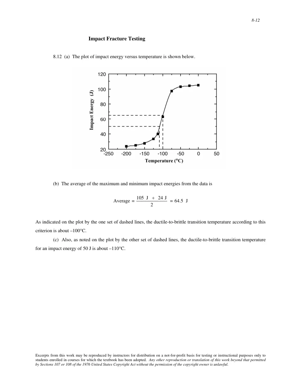8-12 Impact Fracture Testing 8.12 (a) The plot of impact energy versus temperature is shown below. (b) The average of the maximum and minimum impact energies from the data is Average = 105 J + 24 J 2 = 64.5 J As indicated on the plot by the one set of dashed lines, the ductile-to-brittle transition temperature according to this criterion is about –100°C. (c) Also, as noted on the plot by the other set of dashed lines, the ductile-to-brittle transition temperature for an impact energy of 50 J is about –110°C. Excerpts from this work may be reproduced by instructors for distribution on a not-for-profit basis for testing or instructional purposes only to students enrolled in courses for which the textbook has been adopted. Any other reproduction or translation of this work beyond that permitted by Sections 107 or 108 of the 1976 United States Copyright Act without the permission of the copyright owner is unlawful. 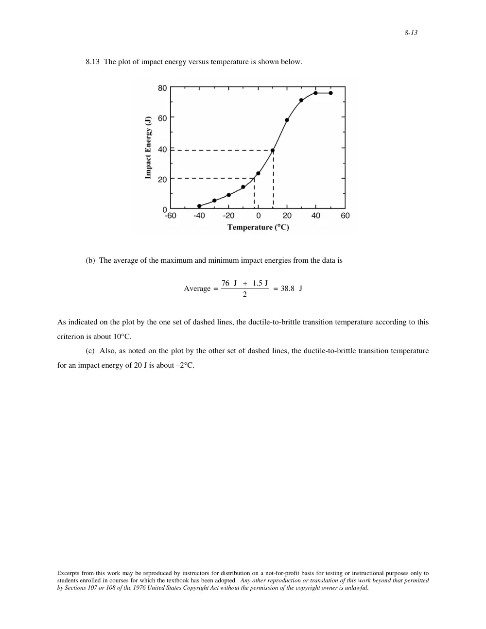8-13 8.13 The plot of impact energy versus temperature is shown below. (b) The average of the maximum and minimum impact energies from the data is Average = 76 J + 1.5 J 2 = 38.8 J As indicated on the plot by the one set of dashed lines, the ductile-to-brittle transition temperature according to this criterion is about 10°C. (c) Also, as noted on the plot by the other set of dashed lines, the ductile-to-brittle transition temperature for an impact energy of 20 J is about –2°C. Excerpts from this work may be reproduced by instructors for distribution on a not-for-profit basis for testing or instructional purposes only to students enrolled in courses for which the textbook has been adopted. Any other reproduction or translation of this work beyond that permitted by Sections 107 or 108 of the 1976 United States Copyright Act without the permission of the copyright owner is unlawful. 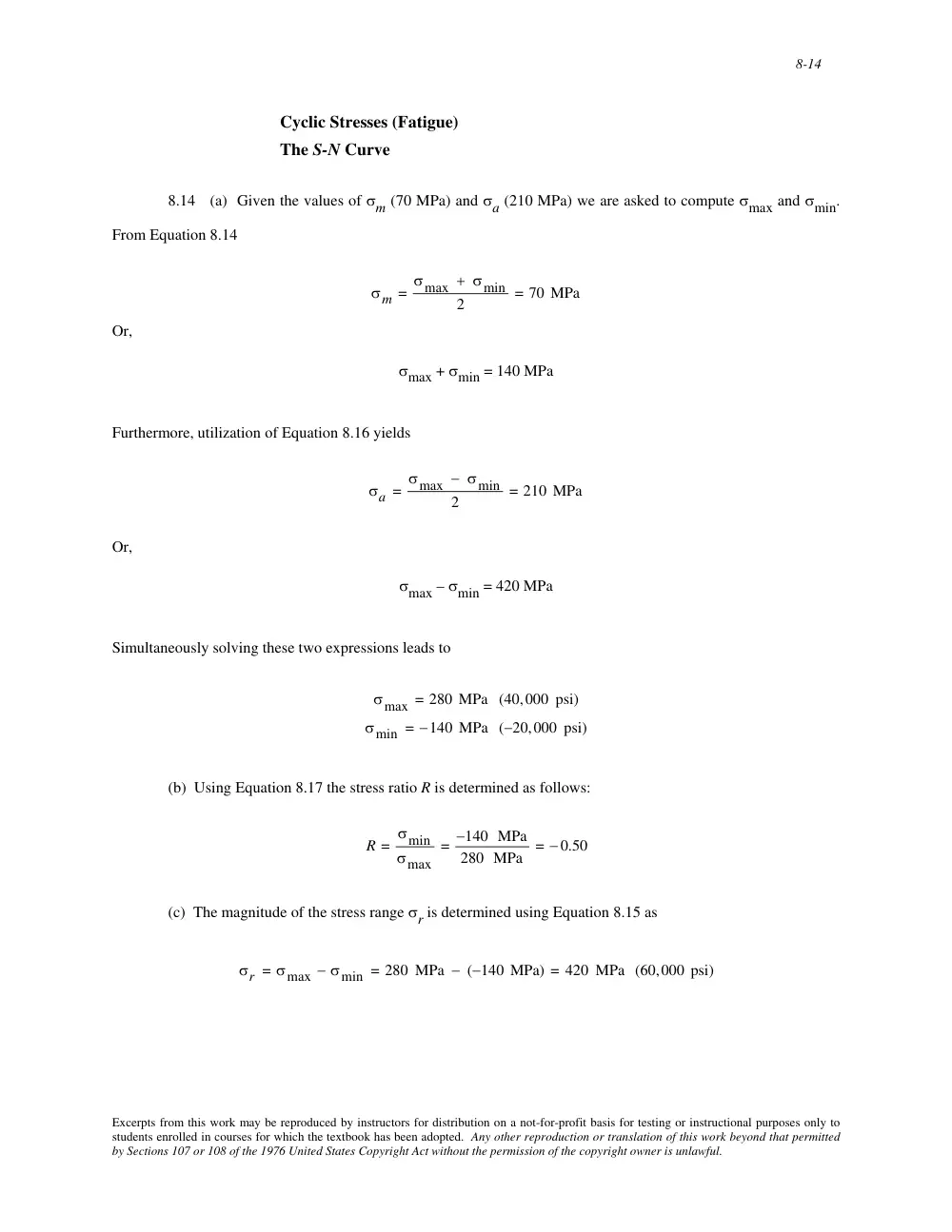8-14 Cyclic Stresses (Fatigue) The S-N Curve 8.14 (a) Given the values of σm (70 MPa) and σa (210 MPa) we are asked to compute σmax and σmin. From Equation 8.14 σm = σmax + σmin 2 = 70 MPa Or, σmax + σmin = 140 MPa Furthermore, utilization of Equation 8.16 yields σa = σmax − σmin 2 = 210 MPa Or, σmax – σmin = 420 MPa Simultaneously solving these two expressions leads to σmax = 280 MPa (40,000 psi) σmin = −140 MPa (−20,000 psi) (b) Using Equation 8.17 the stress ratio R is determined as follows: R = σmin σmax = −140 MPa 280 MPa = − 0.50 (c) The magnitude of the stress range σr is determined using Equation 8.15 as σr = σmax − σmin = 280 MPa − (−140 MPa) = 420 MPa (60,000 psi) Excerpts from this work may be reproduced by instructors for distribution on a not-for-profit basis for testing or instructional purposes only to students enrolled in courses for which the textbook has been adopted. Any other reproduction or translation of this work beyond that permitted by Sections 107 or 108 of the 1976 United States Copyright Act without the permission of the copyright owner is unlawful. 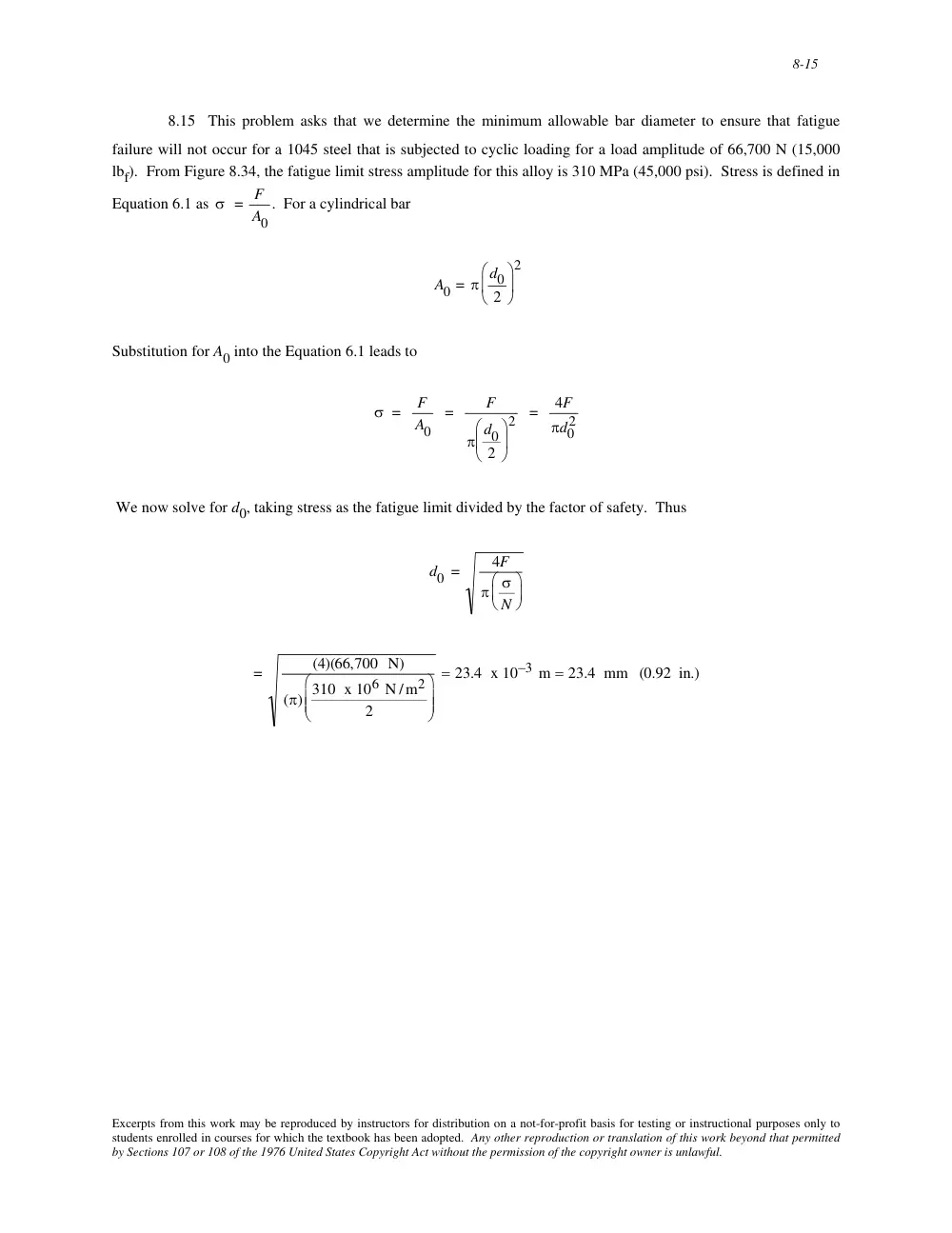8-15 8.15 This problem asks that we determine the minimum allowable bar diameter to ensure that fatigue failure will not occur for a 1045 steel that is subjected to cyclic loading for a load amplitude of 66,700 N (15,000 lbf). From Figure 8.34, the fatigue limit stress amplitude for this alloy is 310 MPa (45,000 psi). Stress is defined in Equation 6.1 as σ = F A0 . For a cylindrical bar A0 = π d0 2 ⎛ ⎝ ⎜ ⎞ ⎠ ⎟ 2 Substitution for A0 into the Equation 6.1 leads to σ = F A0 = F π d0 2 ⎛ ⎝ ⎜ ⎞ ⎠ ⎟ 2 = 4F πd0 2 We now solve for d0, taking stress as the fatigue limit divided by the factor of safety. Thus d0 = 4F π σ N ⎛ ⎝ ⎜ ⎞ ⎠ ⎟ = (4)(66,700 N) (π) 310 x 106 N /m2 2 ⎛ ⎝ ⎜ ⎜ ⎞ ⎠ ⎟ ⎟ = 23.4 x 10−3 m = 23.4 mm (0.92 in.) Excerpts from this work may be reproduced by instructors for distribution on a not-for-profit basis for testing or instructional purposes only to students enrolled in courses for which the textbook has been adopted. Any other reproduction or translation of this work beyond that permitted by Sections 107 or 108 of the 1976 United States Copyright Act without the permission of the copyright owner is unlawful. 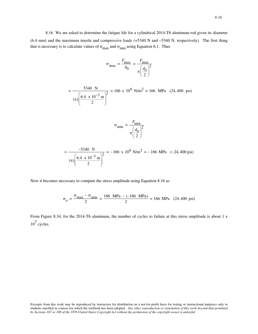8-16 8.16 We are asked to determine the fatigue life for a cylindrical 2014-T6 aluminum rod given its diameter (6.4 mm) and the maximum tensile and compressive loads (+5340 N and –5340 N, respectively). The first thing that is necessary is to calculate values of σmax and σmin using Equation 6.1. Thus σmax = Fmax A0 = Fmax π d0 2 ⎛ ⎝ ⎜ ⎞ ⎠ ⎟ 2 = 5340 N (π) 6.4 x 10−3 m 2 ⎛ ⎝ ⎜ ⎜ ⎞ ⎠ ⎟ ⎟ 2 = 166 x 106 N/m2 = 166 MPa (24,400 psi) σmin = Fmin π d0 2 ⎛ ⎝ ⎜ ⎞ ⎠ ⎟ 2 = −5340 N (π) 6.4 x 10−3 m 2 ⎛ ⎝ ⎜ ⎜ ⎞ ⎠ ⎟ ⎟ 2 = −166 x 106 N/m2 = −166 MPa (−24, 400 psi) Now it becomes necessary to compute the stress amplitude using Equation 8.16 as σa = σmax − σmin 2 = 166 MPa − (−166 MPa) 2 = 166 MPa (24,400 psi) From Figure 8.34, for the 2014-T6 aluminum, the number of cycles to failure at this stress amplitude is about 1 x 107 cycles. Excerpts from this work may be reproduced by instructors for distribution on a not-for-profit basis for testing or instructional purposes only to students enrolled in courses for which the textbook has been adopted. Any other reproduction or translation of this work beyond that permitted by Sections 107 or 108 of the 1976 United States Copyright Act without the permission of the copyright owner is unlawful. 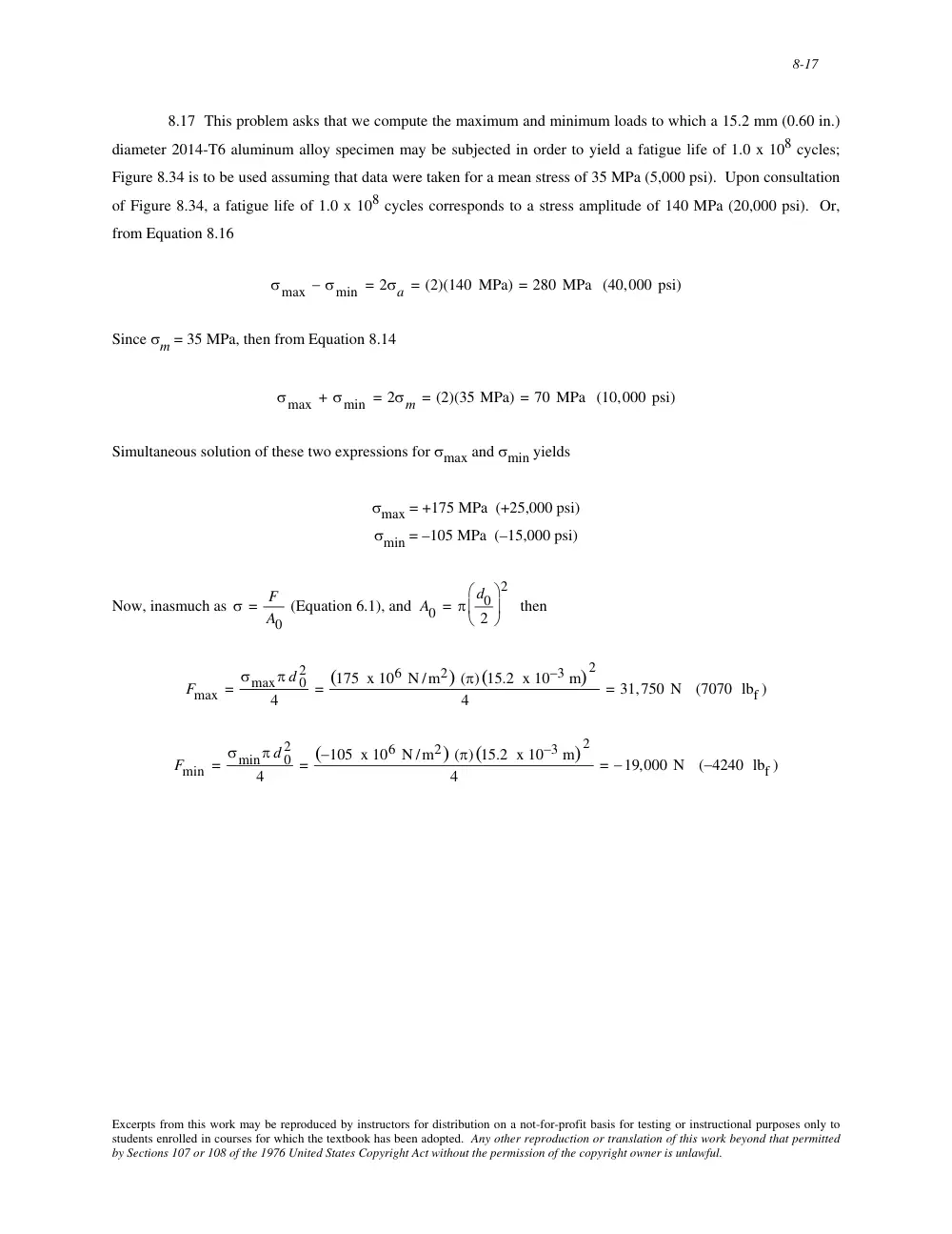8-17 8.17 This problem asks that we compute the maximum and minimum loads to which a 15.2 mm (0.60 in.) diameter 2014-T6 aluminum alloy specimen may be subjected in order to yield a fatigue life of 1.0 x 108 cycles; Figure 8.34 is to be used assuming that data were taken for a mean stress of 35 MPa (5,000 psi). Upon consultation of Figure 8.34, a fatigue life of 1.0 x 108 cycles corresponds to a stress amplitude of 140 MPa (20,000 psi). Or, from Equation 8.16 σmax − σmin = 2σa = (2)(140 MPa) = 280 MPa (40,000 psi) Since σm = 35 MPa, then from Equation 8.14 σmax + σmin = 2σm = (2)(35 MPa) = 70 MPa (10,000 psi) Simultaneous solution of these two expressions for σmax and σmin yields σmax = +175 MPa (+25,000 psi) σmin = –105 MPa (–15,000 psi) Now, inasmuch as σ = F A0 (Equation 6.1), and A0 = π d0 2 ⎛ ⎝ ⎜ ⎞ ⎠ ⎟ 2 then Fmax = σmaxπ d 0 2 4 = (175 x 106 N /m2) (π)(15.2 x 10−3 m) 2 4 = 31,750 N (7070 lbf ) Fmin = σminπ d 0 2 4 = (−105 x 106 N /m2) (π)(15.2 x 10−3 m) 2 4 = −19,000 N (−4240 lbf ) Excerpts from this work may be reproduced by instructors for distribution on a not-for-profit basis for testing or instructional purposes only to students enrolled in courses for which the textbook has been adopted. Any other reproduction or translation of this work beyond that permitted by Sections 107 or 108 of the 1976 United States Copyright Act without the permission of the copyright owner is unlawful. 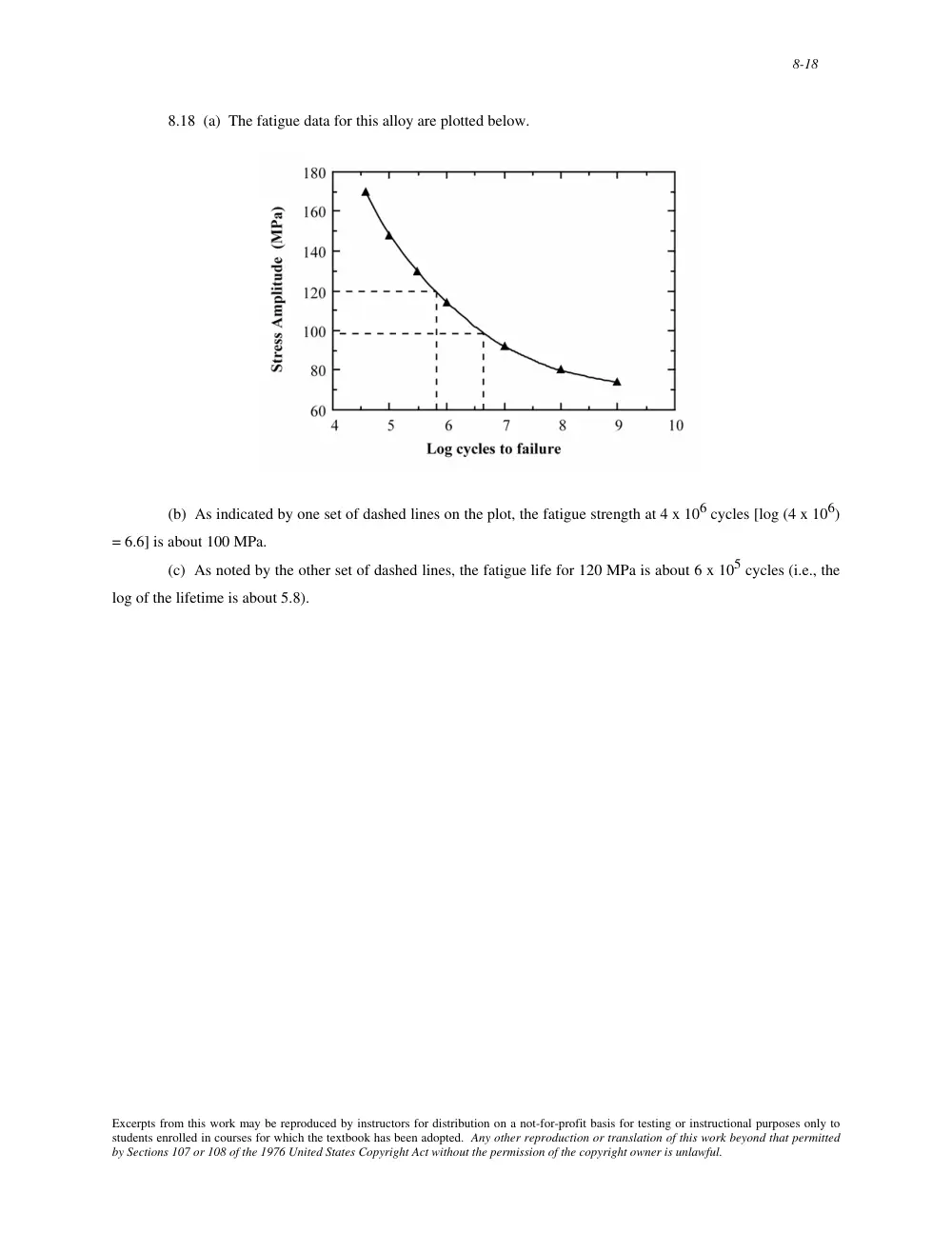8-18 8.18 (a) The fatigue data for this alloy are plotted below. (b) As indicated by one set of dashed lines on the plot, the fatigue strength at 4 x 106 cycles [log (4 x 106) = 6.6] is about 100 MPa. (c) As noted by the other set of dashed lines, the fatigue life for 120 MPa is about 6 x 105 cycles (i.e., the log of the lifetime is about 5.8). Excerpts from this work may be reproduced by instructors for distribution on a not-for-profit basis for testing or instructional purposes only to students enrolled in courses for which the textbook has been adopted. Any other reproduction or translation of this work beyond that permitted by Sections 107 or 108 of the 1976 United States Copyright Act without the permission of the copyright owner is unlawful. 8-19 8.19 We are asked to compute the maximum torsional stress amplitude possible at each of several fatigue lifetimes for the brass alloy the fatigue behavior of which is given in Problem 8.18. For each lifetime, first compute the number of cycles, and then read the corresponding fatigue strength from the above plot. (a) Fatigue lifetime = (1 yr)(365 days/yr)(24 h/day)(60 min/h)(1800 cycles/min) = 9.5 x 108 cycles. The stress amplitude corresponding to this lifetime is about 74 MPa. (b) Fatigue lifetime = (30 days)(24 h/day)(60 min/h)(1800 cycles/min) = 7.8 x 107 cycles. The stress amplitude corresponding to this lifetime is about 80 MPa. (c) Fatigue lifetime = (24 h)(60 min/h)(1800 cycles/min) = 2.6 x 106 cycles. The stress amplitude corresponding to this lifetime is about 103 MPa. (d) Fatigue lifetime = (60 min/h)(1800 cycles/min) = 108,000 cycles. The stress amplitude corresponding to this lifetime is about 145 MPa. Excerpts from this work may be reproduced by instructors for distribution on a not-for-profit basis for testing or instructional purposes only to students enrolled in courses for which the textbook has been adopted. Any other reproduction or translation of this work beyond that permitted by Sections 107 or 108 of the 1976 United States Copyright Act without the permission of the copyright owner is unlawful. 8-2 8.2 In order to estimate the theoretical fracture strength of this material it is necessary to calculate σm using Equation 8.1 given that σ0 = 1035 MPa, a = 0.5 mm, and ρt = 5 x 10-3 mm. Thus, σm = 2σ0 a ρt ⎛ ⎝ ⎜ ⎜ ⎞ ⎠ ⎟ ⎟ 1/2 = (2)(1035 MPa) 0.5 mm 5 x 10−3 mm ⎡ ⎣ ⎢ ⎢ ⎤ ⎦ ⎥ ⎥ 1/2 = 2.07 x 104 MPa = 207 GPa (3 x 106 psi) Excerpts from this work may be reproduced by instructors for distribution on a not-for-profit basis for testing or instructional purposes only to students enrolled in courses for which the textbook has been adopted. Any other reproduction or translation of this work beyond that permitted by Sections 107 or 108 of the 1976 United States Copyright Act without the permission of the copyright owner is unlawful. 8-20 8.20 (a) The fatigue data for this alloy are plotted below. (b) The fatigue limit is the stress level at which the curve becomes horizontal, which is 290 MPa (42,200 psi). (c) From the plot, the fatigue lifetimes at a stress amplitude of 415 MPa (60,000 psi) is about 50,000 cycles (log N = 4.7). At 275 MPa (40,000 psi) the fatigue lifetime is essentially an infinite number of cycles since this stress amplitude is below the fatigue limit. (d) Also from the plot, the fatigue strengths at 2 x 104 cycles (log N = 4.30) and 6 x 105 cycles (log N = 5.78) are 440 MPa (64,000 psi) and 325 MPa (47,500 psi), respectively. Excerpts from this work may be reproduced by instructors for distribution on a not-for-profit basis for testing or instructional purposes only to students enrolled in courses for which the textbook has been adopted. Any other reproduction or translation of this work beyond that permitted by Sections 107 or 108 of the 1976 United States Copyright Act without the permission of the copyright owner is unlawful. 8-21 8.21 This problem asks that we determine the maximum lifetimes of continuous driving that are possible at an average rotational velocity of 600 rpm for the alloy the fatigue data of which is provided in Problem 8.20 and at a variety of stress levels. (a) For a stress level of 450 MPa (65,000 psi), the fatigue lifetime is approximately 18,000 cycles. This translates into (1.8 x 104 cycles)(1 min/600 cycles) = 30 min. (b) For a stress level of 380 MPa (55,000 psi), the fatigue lifetime is approximately 1.5 x 105 cycles. This translates into (1.5 x 105 cycles)(1 min/600 cycles) = 250 min = 4.2 h. (c) For a stress level of 310 MPa (45,000 psi), the fatigue lifetime is approximately 1 x 106 cycles. This translates into (1 x 106 cycles)(1 min/600 cycles) = 1667 min = 27.8 h. (d) For a stress level of 275 MPa (40,000 psi), the fatigue lifetime is essentially infinite since we are below the fatigue limit. Excerpts from this work may be reproduced by instructors for distribution on a not-for-profit basis for testing or instructional purposes only to students enrolled in courses for which the textbook has been adopted. Any other reproduction or translation of this work beyond that permitted by Sections 107 or 108 of the 1976 United States Copyright Act without the permission of the copyright owner is unlawful. 8-22 8.22 For this problem we are given, for three identical fatigue specimens of the same material, σmax and σmin data, and are asked to rank the lifetimes from the longest to the shortest. In order to do this it is necessary to compute both the mean stress and stress amplitude for each specimen. Since from Equation 8.14 σm = σmax + σmin 2 σm(A) = 450 MPa + (−150 MPa) 2 = 150 MPa σm( B) = 300 MPa + (−300 MPa) 2 = 0 MPa σm(C) = 500 MPa + (−200 MPa) 2 = 150 MPa Furthermore, using Equation 8.16 σa = σmax − σmin 2 σa(A) = 450 MPa − (−150 MPa) 2 = 300 MPa σa( B) = 300 MPa − (−300 MPa) 2 = 300 MPa σa(C) = 500 MPa − (−200 MPa) 2 = 350 MPa On the basis of these results, the fatigue lifetime for specimen B will be greater than specimen A which in turn will be greater than specimen C. This conclusion is based upon the following S-N plot on which curves are plotted for two σm values. Excerpts from this work may be reproduced by instructors for distribution on a not-for-profit basis for testing or instructional purposes only to students enrolled in courses for which the textbook has been adopted. Any other reproduction or translation of this work beyond that permitted by Sections 107 or 108 of the 1976 United States Copyright Act without the permission of the copyright owner is unlawful. 8-23 Excerpts from this work may be reproduced by instructors for distribution on a not-for-profit basis for testing or instructional purposes only to students enrolled in courses for which the textbook has been adopted. Any other reproduction or translation of this work beyond that permitted by Sections 107 or 108 of the 1976 United States Copyright Act without the permission of the copyright owner is unlawful. 8-24 8.23 Five factors that lead to scatter in fatigue life data are (1) specimen fabrication and surface preparation, (2) metallurgical variables, (3) specimen alignment in the test apparatus, (4) variation in mean stress, and (5) variation in test cycle frequency. Excerpts from this work may be reproduced by instructors for distribution on a not-for-profit basis for testing or instructional purposes only to students enrolled in courses for which the textbook has been adopted. Any other reproduction or translation of this work beyond that permitted by Sections 107 or 108 of the 1976 United States Copyright Act without the permission of the copyright owner is unlawful. 8-25 Crack Initiation and Propagation Factors That Affect Fatigue Life 8.24 (a) With regard to size, beachmarks are normally of macroscopic dimensions and may be observed with the naked eye; fatigue striations are of microscopic size and it is necessary to observe them using electron microscopy. (b) With regard to origin, beachmarks result from interruptions in the stress cycles; each fatigue striation is corresponds to the advance of a fatigue crack during a single load cycle. Excerpts from this work may be reproduced by instructors for distribution on a not-for-profit basis for testing or instructional purposes only to students enrolled in courses for which the textbook has been adopted. Any other reproduction or translation of this work beyond that permitted by Sections 107 or 108 of the 1976 United States Copyright Act without the permission of the copyright owner is unlawful. 8-26 8.25 Four measures that may be taken to increase the fatigue resistance of a metal alloy are: (1) Polish the surface to remove stress amplification sites. (2) Reduce the number of internal defects (pores, etc.) by means of altering processing and fabrication techniques. (3) Modify the design to eliminate notches and sudden contour changes. (4) Harden the outer surface of the structure by case hardening (carburizing, nitriding) or shot peening. Excerpts from this work may be reproduced by instructors for distribution on a not-for-profit basis for testing or instructional purposes only to students enrolled in courses for which the textbook has been adopted. Any other reproduction or translation of this work beyond that permitted by Sections 107 or 108 of the 1976 United States Copyright Act without the permission of the copyright owner is unlawful. 8-27 Generalized Creep Behavior 8.26 Creep becomes important at about 0.4Tm, Tm being the absolute melting temperature of the metal. (The melting temperatures in degrees Celsius are found inside the front cover of the book.) For Sn, 0.4Tm = (0.4)(232 + 273) = 202 K or -71°C (-96°F) For Mo, 0.4Tm = (0.4)(2617 + 273) = 1156 K or 883°C (1621°F) For Fe, 0.4Tm = (0.4)(1538 + 273) = 724 K or 451°C (845°F) For Au, 0.4Tm = (0.4)(1064 + 273) = 535 K or 262°C (504°F) For Zn, 0.4Tm = (0.4)(420 + 273) = 277 K or 4°C (39°F) For Cr, 0.4Tm = (0.4)(1875 + 273) = 859 K or 586°C (1087°F) Excerpts from this work may be reproduced by instructors for distribution on a not-for-profit basis for testing or instructional purposes only to students enrolled in courses for which the textbook has been adopted. Any other reproduction or translation of this work beyond that permitted by Sections 107 or 108 of the 1976 United States Copyright Act without the permission of the copyright owner is unlawful. 8-28 8.27 These creep data are plotted below The steady-state creep rate (∆ε/∆t) is the slope of the linear region (i.e., the straight line that has been superimposed on the curve) as ∆ε ∆t = 1.20 − 0.25 30 min − 0 min = 3.2 x 10-2 min-1 Excerpts from this work may be reproduced by instructors for distribution on a not-for-profit basis for testing or instructional purposes only to students enrolled in courses for which the textbook has been adopted. Any other reproduction or translation of this work beyond that permitted by Sections 107 or 108 of the 1976 United States Copyright Act without the permission of the copyright owner is unlawful. 8-29 Stress and Temperature Effects 8.28 This problem asks that we determine the total elongation of a low carbon-nickel alloy that is exposed to a tensile stress of 70 MPa (10,000 psi) at 427°C for 10,000 h; the instantaneous and primary creep elongations are 1.3 mm (0.05 in.). From the 427°C line in Figure 8.31, the steady state creep rate Ý ε s is about 4.7 x 10-7 h-1 at 70 MPa. The steady state creep strain, εs, therefore, is just the product of Ý ε s and time as εs = Ý ε s x (time) = (4.7 x 10-7 h-1)(10,000 h) = 4.7 x10-3 Strain and elongation are related as in Equation 6.2; solving for the steady state elongation, ∆ls, leads to ∆ls = l0 εs = (1015 mm)(4.7 x 10-3) = 4.8 mm (0.19 in.) Finally, the total elongation is just the sum of this ∆ls and the total of both instantaneous and primary creep elongations [i.e., 1.3 mm (0.05 in.)]. Therefore, the total elongation is 4.8 mm + 1.3 mm = 6.1 mm (0.24 in.). Excerpts from this work may be reproduced by instructors for distribution on a not-for-profit basis for testing or instructional purposes only to students enrolled in courses for which the textbook has been adopted. Any other reproduction or translation of this work beyond that permitted by Sections 107 or 108 of the 1976 United States Copyright Act without the permission of the copyright owner is unlawful. 8-30 8.29 We are asked to determine the tensile load necessary to elongate a 635 mm long low carbon-nickel alloy specimen 6.44 mm after 5,000 h at 538°C. It is first necessary to calculate the steady state creep rate so that we may utilize Figure 8.31 in order to determine the tensile stress. The steady state elongation, ∆ls, is just the difference between the total elongation and the sum of the instantaneous and primary creep elongations; that is, ∆ls = 6.44 mm − 1.8 mm = 4.64 mm (0.18 in.) Now the steady state creep rate, Ý is just ε s Ý ε s = ∆ε ∆ t = ∆ ls l0 ∆ t = 4.64 mm 635 mm 5,000 h = 1.46 x 10-6 h-1 Employing the 538°C line in Figure 8.31, a steady state creep rate of 1.46 x 10-6 h-1 corresponds to a stress σ of about 40 MPa (5,800 psi) [since log (1.46 x 10-6) = -5.836]. From this we may compute the tensile load using Equation 6.1 as F = σA0 = σπ d0 2 ⎛ ⎝ ⎜ ⎞ ⎠ ⎟ 2 = (40 x 106 N/m2)(π) 19.0 x 10−3 m 2 ⎛ ⎝ ⎜ ⎜ ⎞ ⎠ ⎟ ⎟ 2 = 11,300 N (2560 lbf ) Excerpts from this work may be reproduced by instructors for distribution on a not-for-profit basis for testing or instructional purposes only to students enrolled in courses for which the textbook has been adopted. Any other reproduction or translation of this work beyond that permitted by Sections 107 or 108 of the 1976 United States Copyright Act without the permission of the copyright owner is unlawful. 8-3 8.3 We may determine the critical stress required for the propagation of an internal crack in aluminum oxide using Equation 8.3; taking the value of 393 GPa (Table 12.5) as the modulus of elasticity, we get σc = 2E γs π a ⎡ ⎣ ⎢ ⎤ ⎦ ⎥ 1/2 = (2)(393 x 109 N /m2)(0.90 N /m) (π) 0.4 x 10−3 m 2 ⎛ ⎝ ⎜ ⎜ ⎞ ⎠ ⎟ ⎟ ⎡ ⎣ ⎢ ⎢ ⎢ ⎢ ⎢ ⎤ ⎦ ⎥ ⎥ ⎥ ⎥ ⎥ 1/2 = 33.6 x106 N/m2 = 33.6 MPa Excerpts from this work may be reproduced by instructors for distribution on a not-for-profit basis for testing or instructional purposes only to students enrolled in courses for which the textbook has been adopted. Any other reproduction or translation of this work beyond that permitted by Sections 107 or 108 of the 1976 United States Copyright Act without the permission of the copyright owner is unlawful. 8-31 8.30 This problem asks us to calculate the rupture lifetime of a component fabricated from a low carbon- nickel alloy exposed to a tensile stress of 31 MPa at 649°C. All that we need do is read from the 649°C line in Figure 8.30 the rupture lifetime at 31 MPa; this value is about 10,000 h. Excerpts from this work may be reproduced by instructors for distribution on a not-for-profit basis for testing or instructional purposes only to students enrolled in courses for which the textbook has been adopted. Any other reproduction or translation of this work beyond that permitted by Sections 107 or 108 of the 1976 United States Copyright Act without the permission of the copyright owner is unlawful. 8-32 8.31 We are asked in this problem to determine the maximum load that may be applied to a cylindrical low carbon-nickel alloy component that must survive 10,000 h at 538°C. From Figure 8.30, the stress corresponding to 104 h is about 70 MPa (10,000 psi). Since stress is defined in Equation 6.1 as σ = F/A0, and for a cylindrical specimen, A0 = π d0 2 ⎛ ⎝ ⎜ ⎞ ⎠ ⎟ 2 , then F = σA0 = σπ d0 2 ⎛ ⎝ ⎜ ⎞ ⎠ ⎟ 2 = (70 x 106 N/m2)(π) 19.1 x 10−3 m 2 ⎛ ⎝ ⎜ ⎜ ⎞ ⎠ ⎟ ⎟ 2 = 20,000 N (4420 lbf ) Excerpts from this work may be reproduced by instructors for distribution on a not-for-profit basis for testing or instructional purposes only to students enrolled in courses for which the textbook has been adopted. Any other reproduction or translation of this work beyond that permitted by Sections 107 or 108 of the 1976 United States Copyright Act without the permission of the copyright owner is unlawful. 8-33 8.32 The slope of the line from a log Ý versus log σ plot yields the value of n in Equation 8.19; that is ε s n = ∆ log Ý ε s ∆ log σ We are asked to determine the values of n for the creep data at the three temperatures in Figure 8.31. This is accomplished by taking ratios of the differences between two log Ý ε s and log σ values. (Note: Figure 8.31 plots log σ versus log Ý ; therefore, values of n are equal to the reciprocals of the slopes of the straight-line segments.) ε s Thus for 427°C n = ∆ log Ý ε s ∆ log σ = log (10−6) − log (10−7) log (82 MPa) − log (54 MPa) = 5.5 While for 538°C n = ∆ log Ý ε s ∆ log σ = log 10−5 ( ) − log (10−7) log (59 MPa) − log (22 MPa) = 4.7 And at 649°C n = ∆ log Ý ε s ∆ log σ = log 10−5 ( ) − log (10−7) log (15 MPa) − log (8.3 MPa) = 7.8 Excerpts from this work may be reproduced by instructors for distribution on a not-for-profit basis for testing or instructional purposes only to students enrolled in courses for which the textbook has been adopted. Any other reproduction or translation of this work beyond that permitted by Sections 107 or 108 of the 1976 United States Copyright Act without the permission of the copyright owner is unlawful. 8-34 8.33 (a) We are asked to estimate the activation energy for creep for the low carbon-nickel alloy having the steady-state creep behavior shown in Figure 8.31, using data taken at σ = 55 MPa (8000 psi) and temperatures of 427°C and 538°C. Since σ is a constant, Equation 8.20 takes the form Ý ε s = K2σnexp − Qc RT ⎛ ⎝ ⎜ ⎞ ⎠ ⎟ = K2 ' exp − Qc RT ⎛ ⎝ ⎜ ⎞ ⎠ ⎟ where is now a constant. (Note: the exponent n has about the same value at these two temperatures per Problem 8.32.) Taking natural logarithms of the above expression K2 ' ln Ý ε s = ln K2 ' − Qc RT For the case in which we have creep data at two temperatures (denoted as T1 and T2) and their corresponding steady-state creep rates ( Ý ε s1 and Ý ε s2 ), it is possible to set up two simultaneous equations of the form as above, with two unknowns, namely K2 and Qc. Solving for Qc yields ' Qc = − R ln Ý ε s1 − ln Ý ε s2 ⎛ ⎝ ⎜ ⎞ ⎠ ⎟ 1 T1 − 1 T2 ⎡ ⎣ ⎢ ⎢ ⎤ ⎦ ⎥ ⎥ Let us choose T1 as 427°C (700 K) and T2 as 538°C (811 K); then from Figure 8.31, at σ = 55 MPa, Ý ε s1 = 10-7 h-1 and Ý ε s2 = 8 x 10-6 h-1. Substitution of these values into the above equation leads to Qc = − (8.31 J /mol - K) ln (10−7) − ln (8 x 10−6) [ ] 1 700 K − 1 811 K ⎡ ⎣ ⎢ ⎤ ⎦ ⎥ = 186,200 J/mol (b) We are now asked to estimate Ý ε s at 649°C (922 K). It is first necessary to determine the value of , which is accomplished using the first expression above, the value of Qc, and one value each of K2 ' Ý ε s and T (say Ý ε s1 and T1). Thus, Excerpts from this work may be reproduced by instructors for distribution on a not-for-profit basis for testing or instructional purposes only to students enrolled in courses for which the textbook has been adopted. Any other reproduction or translation of this work beyond that permitted by Sections 107 or 108 of the 1976 United States Copyright Act without the permission of the copyright owner is unlawful. 8-35 K2 ' = Ý ε s1exp Qc RT1 ⎛ ⎝ ⎜ ⎜ ⎞ ⎠ ⎟ ⎟ = 10−7 h−1 ( )exp 186,200 J /mol (8.31 J /mol - K)(700 K) ⎡ ⎣ ⎢ ⎤ ⎦ ⎥ = 8.0 x 106 h-1 Now it is possible to calculate Ý at 649°C (922 K) as follows: ε s Ý ε s = K2 ' exp − Qc RT ⎛ ⎝ ⎜ ⎞ ⎠ ⎟ = 8.0 x 10−6 h−1 ( )exp 186,200 J /mol (8.31 J /mol - K)(922 K) ⎡ ⎣ ⎢ ⎤ ⎦ ⎥ = 2.23 x 10-4 h-1 Excerpts from this work may be reproduced by instructors for distribution on a not-for-profit basis for testing or instructional purposes only to students enrolled in courses for which the textbook has been adopted. Any other reproduction or translation of this work beyond that permitted by Sections 107 or 108 of the 1976 United States Copyright Act without the permission of the copyright owner is unlawful. 8-36 8.34 This problem gives Ý ε s values at two different stress levels and 200°C, and the activation energy for creep, and asks that we determine the steady-state creep rate at 250°C and 48 MPa (7000 psi). Taking natural logarithms of both sides of Equation 8.20 yields ln Ý ε s = ln K2 + n ln σ − Qc RT With the given data there are two unknowns in this equation--namely K2 and n. Using the data provided in the problem statement we can set up two independent equations as follows: ln 2.5 x 10−3 h−1 ( )= ln K2 + n ln(55 MPa) − 140,000 J /mol (8.31 J /mol - K)(473 K) ln 2.4 x 10−2 h−1 ( )= ln K2 + n ln(69 MPa) − 140,000 J /mol (8.31 J /mol - K)(473 K) Now, solving simultaneously for n and K2 leads to n = 9.97 and K2 = 3.27 x 10-5 h-1. Thus it is now possible to solve for Ý at 48 MPa and 523 K using Equation 8.20 as ε s Ý ε s = K2σnexp − Qc RT ⎛ ⎝ ⎜ ⎞ ⎠ ⎟ = 3.27 x 10−5 h−1 ( )(48 MPa)9.97exp − 140,000 J /mo