MAT 315 Useful File

Errors ● True Percent Relative Error: ε t = | true value - approximation | * 100 | true value | ● Approximate Percent Relative Error: ε a = | current approx. - previous approx.| * 100 | current approx. | ● Prespecified Percent Error: ε s = 0.5 * 10 2 - n % where n = desired no. of significant figures Numerical Methods Approximation of ƒ(x) ● Taylor Series Expansion: knowing the value of ƒ(x0) at a certain x0, ƒ(x) where x =% x0 can be approximated using: ƒ(x) = ƒ(x0) + ƒ’(x0)*(x - x0) 1 + ƒ’’(x0)*(x - x0) 2 + ... + ƒ (n) (x 0)*(x - x0) n 1! 2! n! accuracy generally increases as a larger n is chosen Approximation of a Root of a Function ● Bisection Method (Binary Search): x r = x L + x U 2 “sign” = sign of ƒ( x L ) * ƒ( x U ) If sign > 0 : root is between x r and x U , so set new x L = x r and keep x U ( i.e: keep the upper bound x U ) If sign < 0 : root is between x L and x r , so keep x L and set new x U = x r ( i.e: keep the lower bound x L ) ● False Position Method: x r = x U - ƒ( x U )*( x L - x U ) ƒ( x L ) - ƒ( x U ) Similarly, set the new values of xL and xU according to the “sign” of ƒ(xL) * ƒ(xu) ● Simple Fixed Point Method: Requires an initial approximation “x 0” isolate the unknown x to obtain the form: x i+1 = g( x i) In the case of polynomials, start by isolating the highest order term, and then reducing it to x. (this reduces error by reducing exponents) ● Newton-Raphson Method (Tangents): Requires an initial approximation “x0” x i+1 = x i - ƒ( x i) ƒ'( x i) ● Secant Method: Requires 2 initial approximations, “x0” and “x-1” (where x-1 is the value that is more towards the left of the x-axis) x i+1 = x i - ƒ( x i)*( x i-1 - x i) ƒ(x i-1) - ƒ(x i) Approximation of a Root of a Polynomial ● Müller Method: Requires 3 initial approximations “x0”, “x -1”, & “x -2” x i+1 = x i + __-2c_________ b ± sqrt( b2 - 4ac ) where: h 0 = x1 - x0 h 1 = x2 - x2 δ 0 = ƒ( x1 ) - ƒ (x0 ) h 0 δ 1 = ƒ( x2 ) - ƒ( x1 ) h 1 a = δ 1 - δ 0 h 1 + h 0 b = ah 1 + δ 1 c = ƒ( x2 ) For the denominator, choose + or - depending on which yields a larger absolute value. 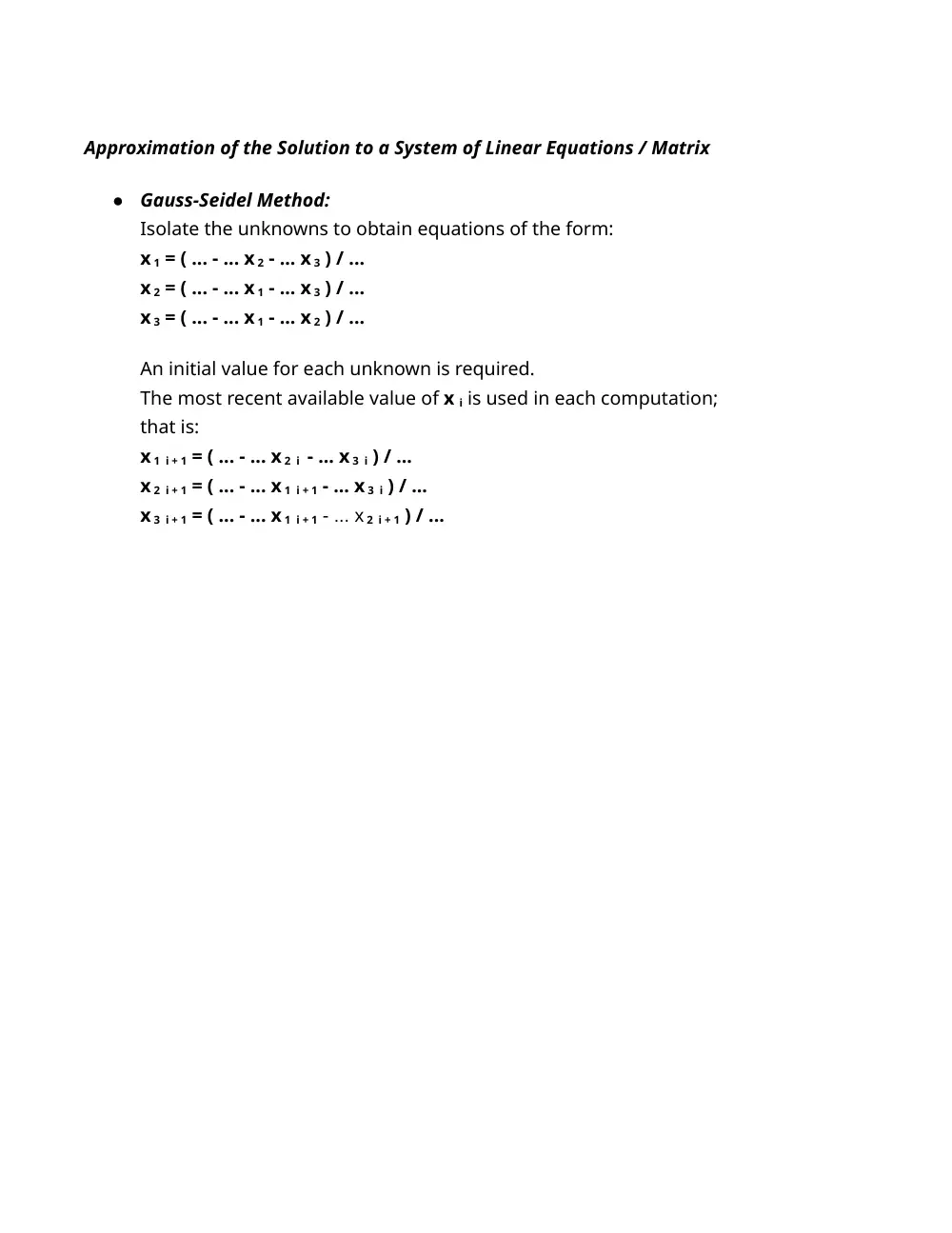Approximation of the Solution to a System of Linear Equations / Matrix ● Gauss-Seidel Method: Isolate the unknowns to obtain equations of the form: x 1 = ( ... - ... x 2 - ... x 3 ) / ... x 2 = ( ... - ... x 1 - ... x 3 ) / ... x 3 = ( ... - ... x 1 - ... x 2 ) / ... An initial value for each unknown is required. The most recent available value of x i is used in each computation; that is: x 1 i + 1 = ( ... - ... x 2 i - ... x 3 i ) / ... x 2 i + 1 = ( ... - ... x 1 i + 1 - ... x 3 i ) / ... x 3 i + 1 = ( ... - ... x 1 i + 1 - ... x 2 i + 1 ) / ... Optimization (Searching for the Minimum/Maximum Points) ● Golden Search Method: golden ratio ≅ 0.618 given an initial range [ x L , x U ] : x 1 = x L + d x 2 = x U - d where d = 0.618 * ( x U - x L ) Note that d > (0.5 * length of range) , which means the points are in this order: x L ____ x 2 _______ x 1 ____ x U [_______ d _______] To reduce the range for the next iteration (when searching for max pt. ): - if ƒ( x 1 ) > ƒ( x 2 ) , then x 1 is optimal (closer to the max pt), so the new range is [ x 2 , x U ] - if ƒ( x 1 ) < ƒ( x 2 ) , then x 2 is optimal (closer to the max pt), so the new range is [ x L , x 1 ] Note that the min pt. of ƒ(x) is equivalent to the max pt. of - ƒ(x) When using this method, Approximate Percent Relative Error is found by: ε a = 0.382 * | ( x U - x L ) / x optimal | * 100 ● Newton Method: Requires an initial approximation “x 0” x i + 1 = x i - ƒ’( x i) ƒ’‘( x i) If ƒ”( x ) > 0 : min pt. If ƒ”( x ) < 0 : max pt. 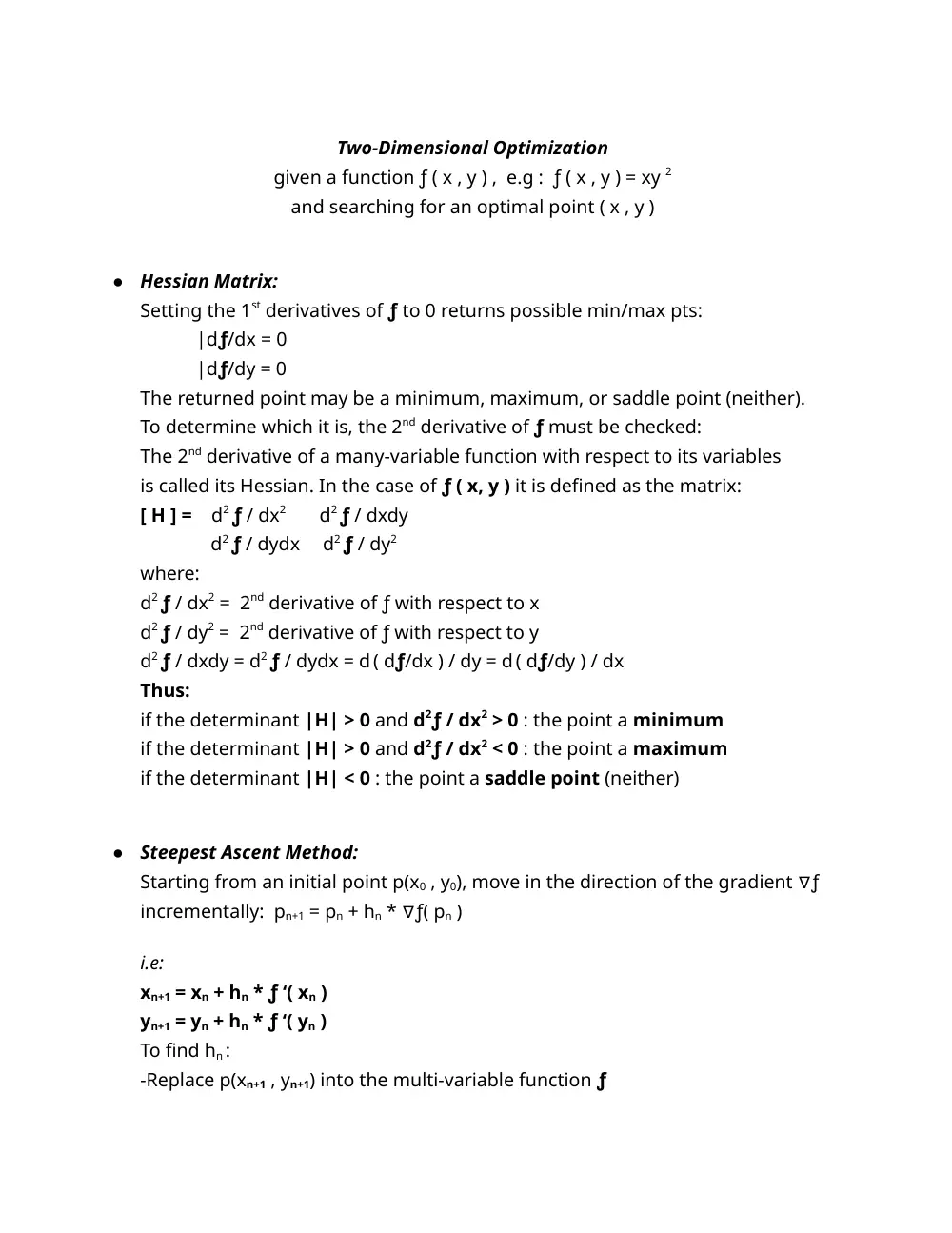Two-Dimensional Optimization given a function ƒ ( x , y ) , e.g : ƒ ( x , y ) = xy 2 and searching for an optimal point ( x , y ) ● Hessian Matrix: Setting the 1st derivatives of ƒ to 0 returns possible min/max pts: |dƒ/dx = 0 |dƒ/dy = 0 The returned point may be a minimum, maximum, or saddle point (neither). To determine which it is, the 2nd derivative of ƒ must be checked: The 2nd derivative of a many-variable function with respect to its variables is called its Hessian. In the case of ƒ ( x, y ) it is defined as the matrix: [ H ] = d2 ƒ / dx2 d2 ƒ / dxdy d2 ƒ / dydx d2 ƒ / dy2 where: d2 ƒ / dx2 = 2nd derivative of ƒ with respect to x d2 ƒ / dy2 = 2nd derivative of ƒ with respect to y d2 ƒ / dxdy = d2 ƒ / dydx = d ( dƒ/dx ) / dy = d ( dƒ/dy ) / dx Thus: if the determinant |H| > 0 and d2ƒ / dx2 > 0 : the point a minimum if the determinant |H| > 0 and d2ƒ / dx2 < 0 : the point a maximum if the determinant |H| < 0 : the point a saddle point (neither) ● Steepest Ascent Method: Starting from an initial point p(x0 , y0), move in the direction of the gradient ∇ƒ incrementally: pn+1 = pn + hn * ∇ƒ( pn ) i.e: xn+1 = xn + hn * ƒ ‘( xn ) yn+1 = yn + hn * ƒ ‘( yn ) To find hn : -Replace p(xn+1 , yn+1) into the multi-variable function ƒ 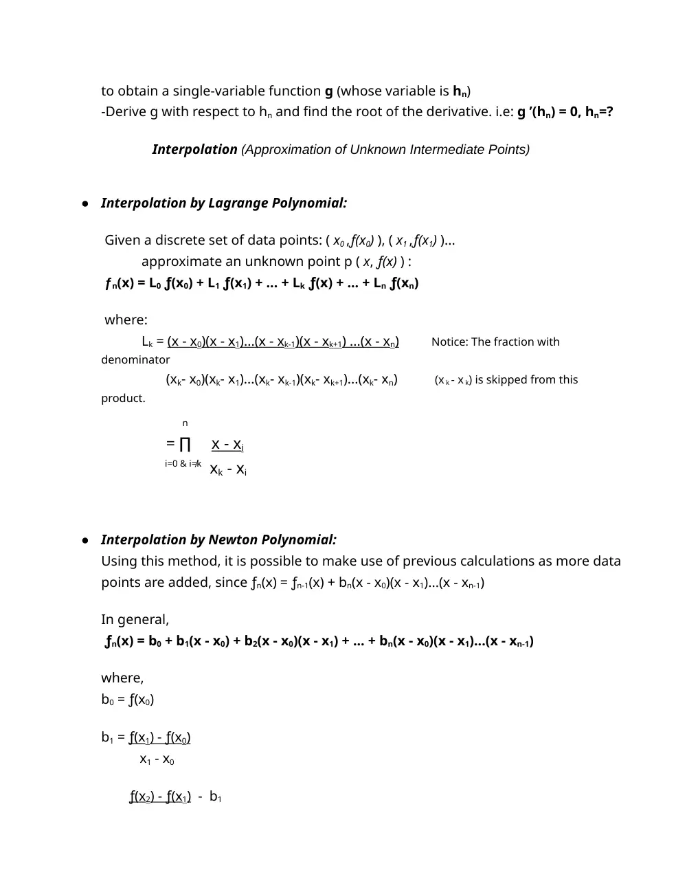to obtain a single-variable function g (whose variable is hn) -Derive g with respect to hn and find the root of the derivative. i.e: g ’(hn) = 0, hn=? Interpolation (Approximation of Unknown Intermediate Points) ● Interpolation by Lagrange Polynomial: Given a discrete set of data points: ( x0 ,ƒ(x0) ), ( x1 ,ƒ(x1) )... approximate an unknown point p ( x, ƒ(x) ) : ƒn(x) = L0 ƒ(x0) + L1 ƒ(x1) + ... + Lk ƒ(x) + ... + Ln ƒ(xn) where: Lk = (x - x0)(x - x1)...(x - xk-1)(x - xk+1) ...(x - xn) Notice: The fraction with denominator (xk- x0)(xk- x1)...(xk- xk-1)(xk- xk+1)...(xk- xn) (x k - x k) is skipped from this product. n = ∏ x - xi i=0 & i=%k xk - xi ● Interpolation by Newton Polynomial: Using this method, it is possible to make use of previous calculations as more data points are added, since ƒn(x) = ƒn-1(x) + bn(x - x0)(x - x1)...(x - xn-1) In general, ƒn(x) = b0 + b1(x - x0) + b2(x - x0)(x - x1) + ... + bn(x - x0)(x - x1)...(x - xn-1) where, b0 = ƒ(x0) b1 = ƒ(x1) - ƒ(x0) x1 - x0 ƒ(x2) - ƒ(x1) - b1 b2 = x2 - x1 and in general: bn = D n-1 ƒ 1 - D n-1 ƒ 0 = Dnƒ0 x2 - x0 xn - x0 (where Dƒ is known as the “divided difference”) Approximation of Integrals xn given an integral ∫ƒ(x) dx x0 and given that the interval [x0 , xn] is divided into N segments of equal length let h = (xn - x0) N Note that h is the distance between successive abscissas x0 & x1, x1 & x2, etc. ƒ(xn) is denoted as ƒn for brevity in the following ● Trapezoidal Rule: xn ∫ƒ(x) dx = h { (ƒ0 + ƒ1) + (ƒ1 + ƒ2) + ... + (ƒn-2 + ƒn-1) + (ƒn-1 + ƒn) } x0 2 i.e: xn ∫ƒ(x) dx = h ( ƒ0 + 2ƒ1 + 2ƒ2 + ... + 2ƒn-2 + 2ƒn-1 + ƒn) x0 2 ● Simpson’s 1/3 Rule: Simpson’s rules are generally significantly more accurate than the trapezoidal rule. Assuming n is even: xn ∫ƒ(x)dx = h{(ƒ0 +4ƒ1 + ƒ2) + (ƒ2 +4ƒ3 + ƒ4) +...+ (ƒn-4 +4ƒn-3 + ƒn-2) + (ƒn-2 +4ƒn-1 + ƒn)} x0 3 i.e: xn ∫ƒ(x)dx = h (ƒ0 + 4ƒ1 + 2ƒ2 + 4ƒ3 + 2ƒ4 +...+ 2ƒn-4 + 4ƒn-3 + 2ƒn-2 + 4ƒn-1 + ƒn) x0 3 i.e: xn ∫ƒ(x)dx = h ( ƒ0 + 4∑ƒodd-numbers + 2∑ƒeven-numbers + ƒn ) x0 3 ● Simpson’s 3/8 Rule: Has a fixed formula; fixed at N = 3 and n = 3: h = x3 - x0 3 x3 ∫ƒ(x)dx = 3h ( ƒ0 + 3ƒ1 + 3ƒ2 + ƒ3 ) x0 8 ● 2-Point Gauss-Legendre: The interval of the integral must be [-1,1 ] If it is not, any definite integral can be changed to an integral over [-1,1 ] using a variable substitution known as Gauss-Legendre translation: xnew = (xn - x0) xold + (xn + x0) 2 2 dxnew = (xn - x0) dxold 2 i.e: xn 1 1 ∫ƒ(x) dx = (xn - x0) ∫ƒ( (xn - x0) x + (xn + x0) ) dx = ∫ƒ(xnew) dxnew x0 2 -1 2 2 -1 The 2-Point Gauss Legendre formula can now be applied: 1 ∫ƒ(x) dx = f( -1 ) + f( 1 ) -1 ( 3 ) √ ( 3 ) √ This approximation formula actually gives the exact result for polynomials of degree ≤ 3 Approximation of Solutions of Ordinary Differential Equations given y'(t) = ƒ(t, y) (i.e. ƒ denotes the 1st derivative) and y(t0) = y0 as well as a step size h, where h is also the difference between successive tn-1 & tn ● Euler’s Method: Low accuracy yn+1 = yn + hƒ(tn, yn) ● Midpoint Method: High accuracy yn+1 = yn + k2 h where: k1 = ƒ(xn, yn) k2 = ƒ(xn + h , yn + k1 h ) 2 2 ● Runge-Kutta Method: Less accurate than Midpoint Method yn+1 = yn + ( k1 + k2 ) h 2 2 where: k1 = ƒ(xn, yn) k2 = ƒ(xn + h , yn + k1 h )