EEN 330 Problems Chapter 5, Spring 2012

233 Chapter 5: Magnetostatics Lesson #30 Chapter — Section: 5-1 Topics: Magnetic forces and torques Highlights: • Lorentz force on a charged particle • Magnetic force on a current in a magnetic field • Torque on a loop Special Illustrations: • Examples 5-1 234 Lesson #31 Chapter — Section: 5-2 Topics: Biot-Savart law Highlights: • Magnetic field induction by electric currents • Magnetic field due to linear conductor • Magnetic dipole Special Illustrations: • 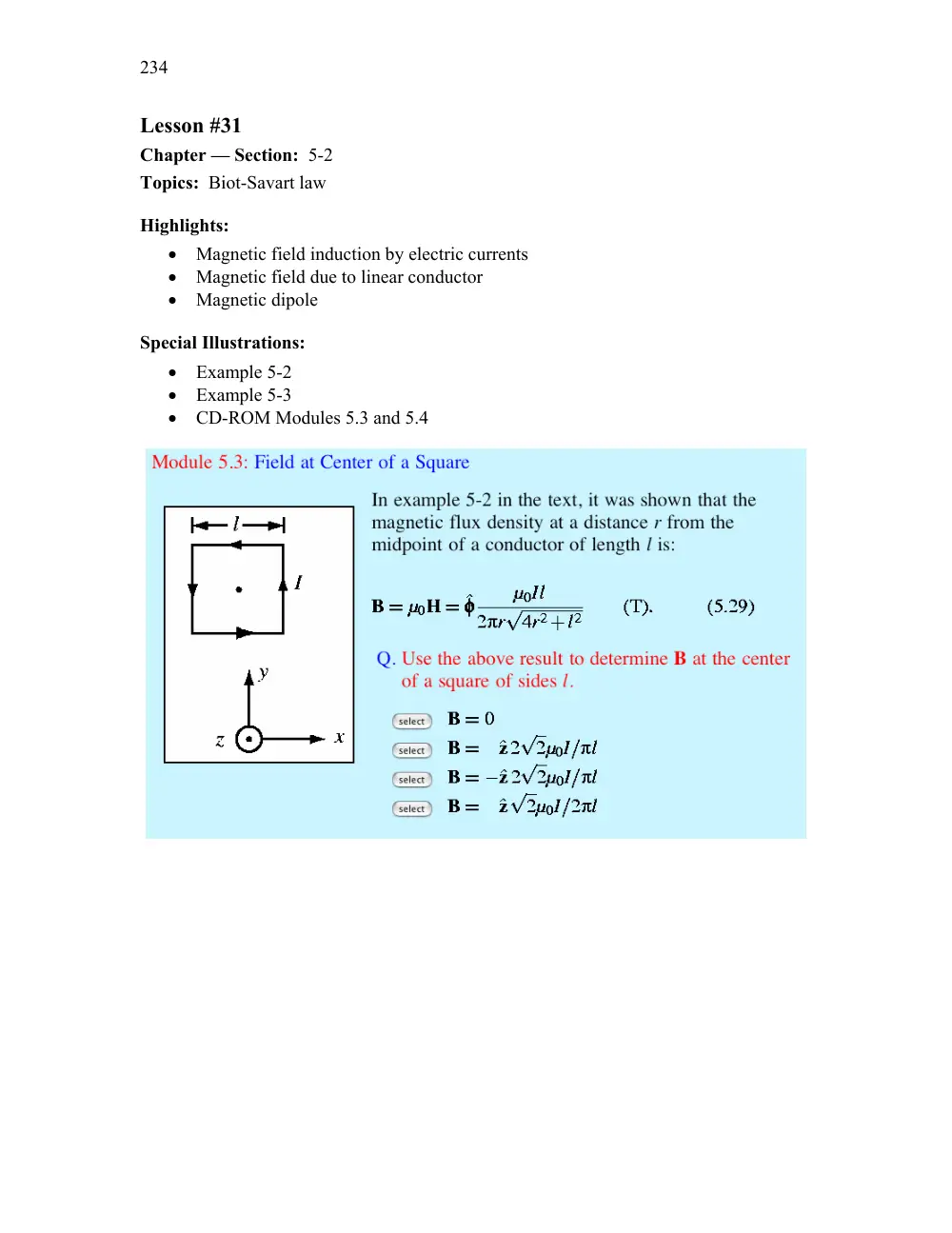Example 5-2 • Example 5-3 • CD-ROM Modules 5.3 and 5.4 235 Lesson #32 Chapter — Section: 5-3, 5-4 Topics: Magnetic force, Ampère’s law Highlights: • Attraction and repulsion forces between currents • Gauss’s law for magnetics • Ampère’s law Special Illustrations: • Example 5-6 • CD-ROM Modules 5.1 and 5.2 236 Lesson #33 Chapter — Section: 5-5, 5-6 Topics: Vector magnetic potential, magnetic materials Highlights: • Relation of A to B • Vector Poisson’s Eq. • Magnetic permeability • Ferromagnetism, hysteresis Special Illustrations: • Technology Brief on “Electromagnetic and magnetic switches” (CD-ROM) Electromagnets and Magnetic Relays William Sturgeon developed the first practical electromagnet in the 1820s. Today the principle of the electromagnet is used in motors, relay switches in read/write heads for hard disks and tape drives, loudspeakers, magnetic levitation and many other applications. 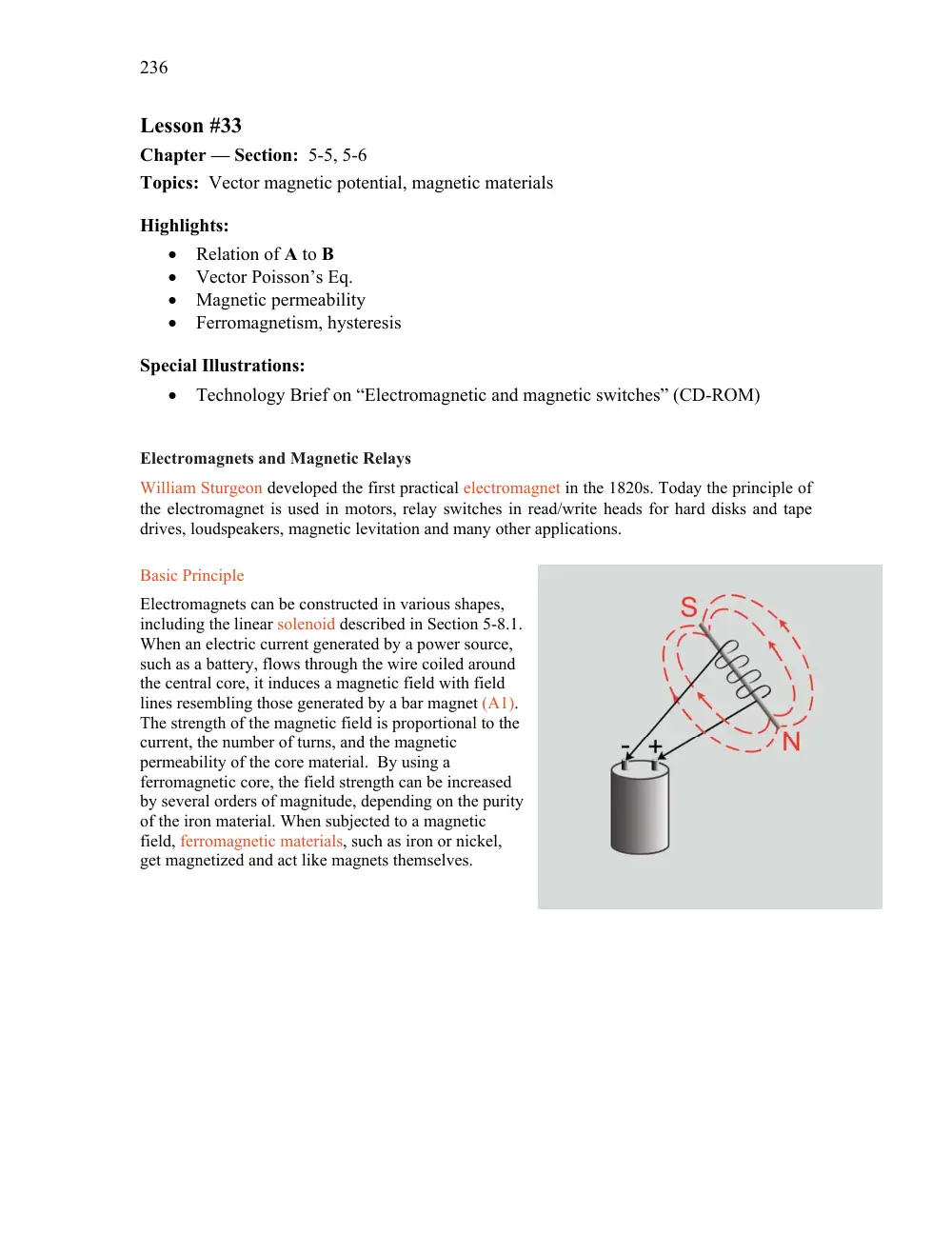Basic Principle Electromagnets can be constructed in various shapes, including the linear solenoid described in Section 5-8.1. When an electric current generated by a power source, such as a battery, flows through the wire coiled around the central core, it induces a magnetic field with field lines resembling those generated by a bar magnet (A1). The strength of the magnetic field is proportional to the current, the number of turns, and the magnetic permeability of the core material. By using a ferromagnetic core, the field strength can be increased by several orders of magnitude, depending on the purity of the iron material. When subjected to a magnetic field, ferromagnetic materials, such as iron or nickel, get magnetized and act like magnets themselves. 237 Lesson #34 Chapter — Section: 5-7 Topics: Boundary conditions Highlights: • Analogy with electric-field boundary conditions Special Illustrations: • Technology Brief on “Magnetic Recording” (CD-ROM) Magnetic Recording Valdemar Poulsen, a Danish engineer, invented magnetic recording by demonstrating in 1900 that speech can be recorded on a thin steel wire using a simple electromagnet. Magnetic tapes were developed as an alternative medium to wires in the 1940s and became very popular for recording and playing music well into the 1960s. Videotapes were introduced in the late 1950s for recording motion pictures for later replay on television. Because video signals occupy a much wider bandwidth, tape speeds for video recording (past the magnetic head) have to be at rates on the order of 5 m/s, compared with only 0.3 m/s for audio. Other types of magnetic recording media were developed since then, including the flexible plastic disks called “floppies,” the hard disks made of glass or aluminum, the magnetic drum, and the magnetic bubble memory. All take advantage of the same fundamental principle of being able to store electrical information through selective magnetization of a magnetic material, as well as the ability to retrieve it (playback) when so desired. 238 Lesson #35 Chapter — Section: 5-8 Topics: Inductance Highlights: • Solenoid • Self inductance Special Illustrations: • Example 5-8 • Technology Brief on “Inductive Sensors” (CD-ROM) Inductive Sensors Magnetic coupling between different coils forms the basis of several different types of inductive sensors. Applications include the measurement of position and displacement (with sub-millimeter resolution) in device fabrications processes, proximity detection of conductive objects, and other related applications. 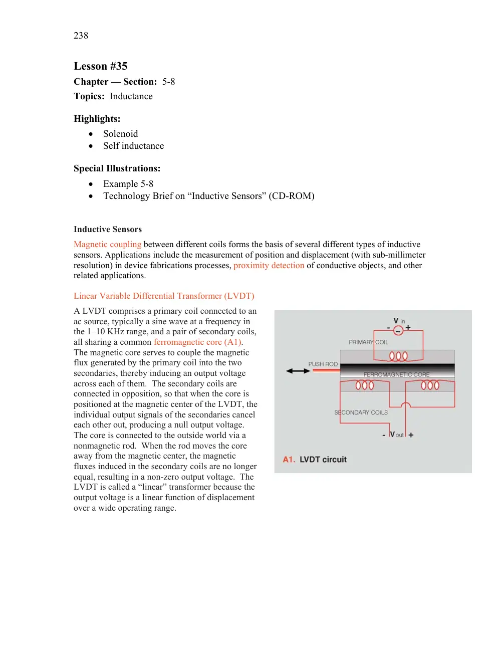Linear Variable Differential Transformer (LVDT) A LVDT comprises a primary coil connected to an ac source, typically a sine wave at a frequency in the 1–10 KHz range, and a pair of secondary coils, all sharing a common ferromagnetic core (A1). The magnetic core serves to couple the magnetic flux generated by the primary coil into the two secondaries, thereby inducing an output voltage across each of them. The secondary coils are connected in opposition, so that when the core is positioned at the magnetic center of the LVDT, the individual output signals of the secondaries cancel each other out, producing a null output voltage. The core is connected to the outside world via a nonmagnetic rod. When the rod moves the core away from the magnetic center, the magnetic fluxes induced in the secondary coils are no longer equal, resulting in a non-zero output voltage. The LVDT is called a “linear” transformer because the output voltage is a linear function of displacement over a wide operating range. 239 Lesson #36 Chapter — Section: 5-9 Topics: Magnetic energy Highlights: • Magnetic energy density • Magnetic energy in a coax Special Illustrations: • Example 5-9 240 CHAPTER 5 Chapter 5 Sections 5-1: Forces and Torques Problem 5.1 An electron with a speed of 8 106 m/s is projected along the positive x-direction into a medium containing a uniform magnetic flux density B � � ˆx4 � ˆz3 � T. Given that e � 1 6 10  19 C and the mass of an electron is me � 9 1 10  31 kg, determine the initial acceleration vector of the electron (at the moment it is projected into the medium). Solution: The acceleration vector of a free particle is the net force vector divided by the particle mass. Neglecting gravity, and using Eq. 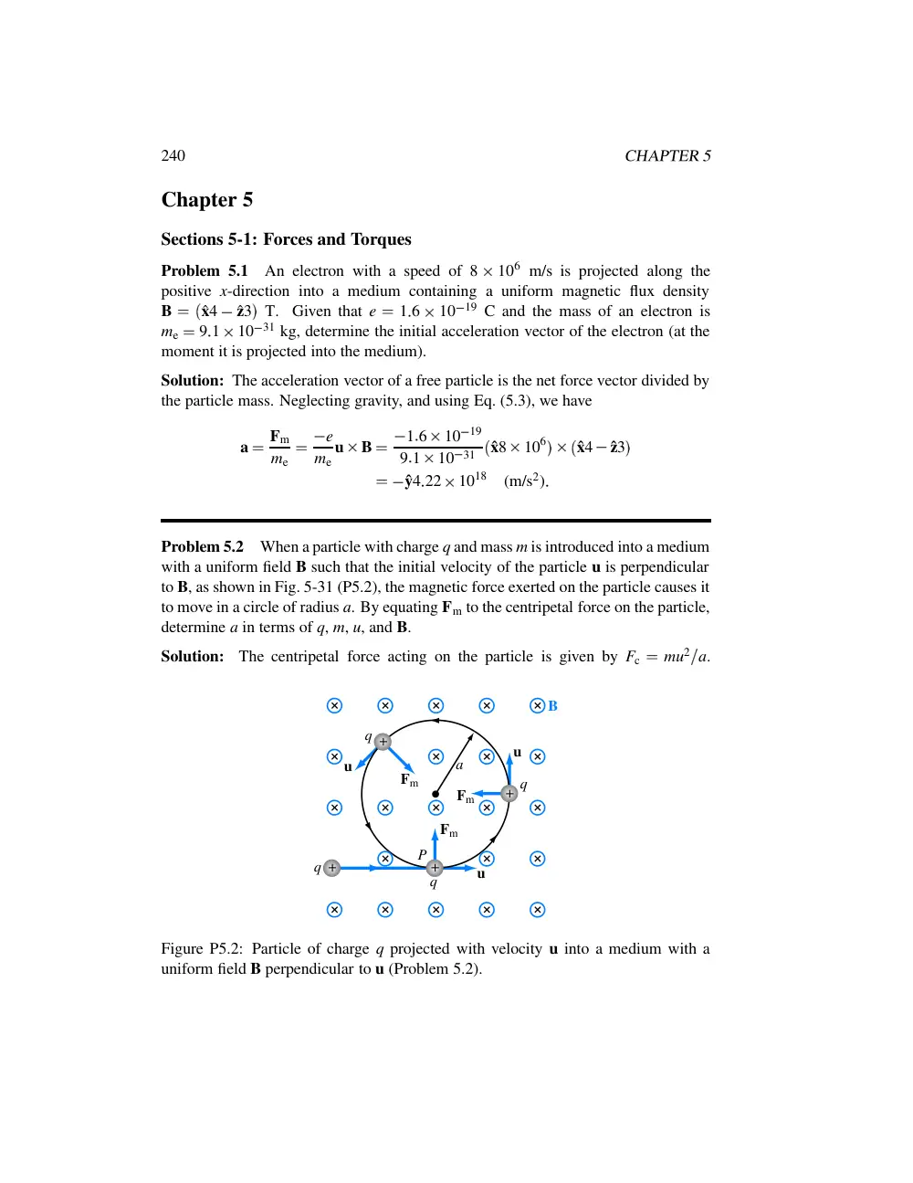(5.3), we have a � Fm me � � e me u B � � 1 6 10  19 9 1 10  31 � ˆx8 106 �� � ˆx4 � ˆz3 � � � ˆy4 22 1018 (m/s2) Problem 5.2 When a particle with charge q and mass m is introduced into a medium with a uniform field B such that the initial velocity of the particle u is perpendicular to B, as shown in Fig. 5-31 (P5.2), the magnetic force exerted on the particle causes it to move in a circle of radius a. By equating Fm to the centripetal force on the particle, determine a in terms of q, m, u, and B. Solution: The centripetal force acting on the particle is given by Fc � mu2 a. Fm Fm B Fm + + + + q a q q q u u u P Figure P5.2: Particle of charge q projected with velocity u into a medium with a uniform field B perpendicular to u (Problem 5.2). CHAPTER 5 241 Equating Fc to Fm given by Eq. (5.4), we have mu2 a � quBsinθ. Since the magnetic field is perpendicular to the particle velocity, sinθ � 1. Hence, a � mu qB. 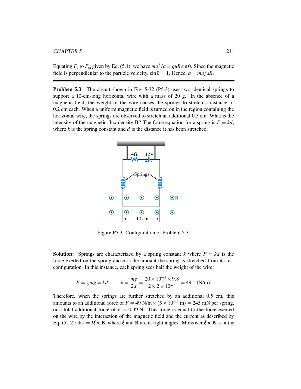Problem 5.3 The circuit shown in Fig. 5-32 (P5.3) uses two identical springs to support a 10-cm-long horizontal wire with a mass of 20 g. In the absence of a magnetic field, the weight of the wire causes the springs to stretch a distance of 0.2 cm each. When a uniform magnetic field is turned on in the region containing the horizontal wire, the springs are observed to stretch an additional 0.5 cm. What is the intensity of the magnetic flux density B? The force equation for a spring is F � kd, where k is the spring constant and d is the distance it has been stretched. 4Ω 12V B 10 cm Springs + - Figure P5.3: Configuration of Problem 5.3. Solution: Springs are characterized by a spring constant k where F � kd is the force exerted on the spring and d is the amount the spring is stretched from its rest configuration. In this instance, each spring sees half the weight of the wire: F � 1 2mg � kd � k � mg 2d � 20 10  3 9 8 2 2 10  3 � 49 (N/m) Therefore, when the springs are further stretched by an additional 0.5 cm, this amounts to an additional force of F � 49 N/m � 5 10  3 m �� 245 mN per spring, or a total additional force of F � 0 49 N. This force is equal to the force exerted on the wire by the interaction of the magnetic field and the current as described by Eq. (5.12): Fm � I � � � B, where � � � and B are at right angles. Moreover � � � B is in the 242 CHAPTER 5 downward direction, and I � V R � 12 V 4 Ω � 3 A. 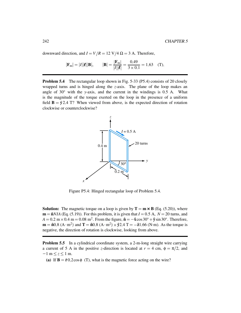Therefore, � Fm � � � I � � � � � � � B � � � B � � � Fm � � I � � � � � � � 0 49 3 0 1 � 1 63 (T) Problem 5.4 The rectangular loop shown in Fig. 5-33 (P5.4) consists of 20 closely wrapped turns and is hinged along the z-axis. The plane of the loop makes an angle of 30 � with the y-axis, and the current in the windings is 0.5 A. What is the magnitude of the torque exerted on the loop in the presence of a uniform field B � ˆy2 4 T? When viewed from above, is the expected direction of rotation clockwise or counterclockwise? 30° 0.4 m 0.2 m y x z I = 0.5 A 20 turns Figure P5.4: Hinged rectangular loop of Problem 5.4. Solution: The magnetic torque on a loop is given by T � m B (Eq. (5.20)), where m � ˆnNIA (Eq. (5.19)). For this problem, it is given that I � 0 5 A, N � 20 turns, and A � 0 2 m 0 4 m � 0 08 m2. From the figure, ˆn � � ˆxcos30 � � ˆysin30 � . Therefore, m � ˆn0 8 (A � m2 � and T � ˆn0 8 (A � m2 �� ˆy2 4 T � � ˆz1 66 (N � m). As the torque is negative, the direction of rotation is clockwise, looking from above. Problem 5.5 In a cylindrical coordinate system, a 2-m-long straight wire carrying a current of 5 A in the positive z-direction is located at r � 4 cm, φ � π 2, and � 1 m � z � 1 m. (a) If B � ˆr0 2cosφ (T), what is the magnetic force acting on the wire? CHAPTER 5 243 z y -1 m 1 m 4 cm 5A Figure P5.5: Problem 5.5. (b) How much work is required to rotate the wire once about the z-axis in the negative φ-direction (while maintaining r � 4 cm)? (c) At what angle φ is the force a maximum? Solution: (a) F � I � � � B � 5ˆz2 � ˆr0 2cosφ � � ˆφφφ2cosφ At φ � π 2, ˆφφφ � � ˆx. Hence, F � � ˆx2cos � π 2 �� 0 (b) W � � 2π φ � 0 F � dl � � 2π 0 ˆφφφ � 2cosφ � � � � ˆφφφ � r dφ � � � � r � 4 cm � � 2r � 2π 0 cosφdφ � � � � r � 4 cm � � 8 10  2 � sinφ� 2π 0 � 0 The force is in the � ˆφφφ-direction, which means that rotating it in the � ˆφφφ-direction would require work. However, the force varies as cosφ, which means it is positive 244 CHAPTER 5 when � π 2 � φ � π 2 and negative over the second half of the circle. Thus, work is provided by the force between φ � π 2 and φ � � π 2 (when rotated in the � ˆφφφ-direction), and work is supplied for the second half of the rotation, resulting in a net work of zero. (c) The force F is maximum when cosφ � 1, or φ � 0. Problem 5.6 A 20-turn rectangular coil with side l � 20 cm and w � 10 cm is placed in the y–z plane as shown in Fig. 5-34 (P5.6). φ z y x l w I n^ 20-turn coil Figure P5.6: Rectangular loop of Problem 5.6. (a) If the coil, which carries a current I � 10 A, is in the presence of a magnetic flux density B � 2 10  2 � ˆx � ˆy2 � (T) � determine the torque acting on the coil. (b) At what angle φ is the torque zero? (c) At what angle φ is the torque maximum? Determine its value. Solution: (a) The magnetic field is in direction � ˆx � ˆy2 � , which makes an angle φ0 � tan  1 2 1 � 63 43 � . The magnetic moment of the loop is m � ˆnNIA � ˆn20 10 � 30 10 �� 10  4 � ˆn6 (A � m2) � CHAPTER 5 245 1 2 z y B x φ0 = 63.43o Figure P5.6: (a) Direction of B. where ˆn is the surface normal in accordance with the right-hand rule. When the loop is in the negative-y of the y–z plane, ˆn is equal to ˆx, but when the plane of the loop is moved to an angle φ, ˆn becomes ˆn � ˆxcosφ � ˆysinφ � T � m B � ˆn6 2 10  2 � ˆx � ˆy2 � � � ˆxcosφ � ˆysinφ � 6 2 10  2 � ˆx � ˆy2 � � ˆz0 12 � 2cosφ � sinφ� (N � m) (b) The torque is zero when 2cosφ � sinφ � 0 � or tanφ � 2 � φ � 63 43 � or � 116 57 � Thus, when ˆn is parallel to B, T � 0. (c) The torque is a maximum when ˆn is perpendicular to B, which occurs at φ � 63 43 � 90 � � � 26 57 � or � 153 43 � Mathematically, we can obtain the same result by taking the derivative of T and equating it to zero to find the values of φ at which � T � is a maximum. Thus, ∂T ∂φ � ∂ ∂φ � 0 12 � 2cosφ � sinφ � �� 0 246 CHAPTER 5 or � 2sinφ � cosφ � 0 � which gives tanφ � � 1 2 , or φ � � 26 57 � or 153 43 � � at which T � ˆz0 27 (N � m). Section 5-2: Biot–Savart Law Problem 5.7 An 8 cm 12 cm rectangular loop of wire is situated in the x–y plane with the center of the loop at the origin and its long sides parallel to the x-axis. The loop has a current of 50 A flowing with clockwise direction (when viewed from above). Determine the magnetic field at the center of the loop. Solution: The total magnetic field is the vector sum of the individual fields of each of the four wire segments: B � B1 � B2 � B3 � B4. An expression for the magnetic field from a wire segment is given by Eq. (5.29). -4 cm 4 cm -6 cm 6 cm y x I z 4 3 2 1 Figure P5.7: Problem 5.7. For all segments shown in Fig. P5.7, the combination of the direction of the current and the right-hand rule gives the direction of the magnetic field as � z direction at the origin. With r � 6 cm and l � 8 cm, B1 � � ˆz µIl 2πr � 4r2 � l2 � � ˆz 4π 10  7 50 0 08 2π 0 06 � 4 0 062 � 0 082 � � ˆz9 24 10  5 (T) CHAPTER 5 247 For segment 2, r � 4 cm and l � 12 cm, B2 � � ˆz µIl 2πr � 4r2 � l2 � � ˆz 4π 10  7 50 0 12 2π 0 04 � 4 0 042 � 0 122 � � ˆz20 80 10  5 (T) Similarly, B3 � � ˆz9 24 10  5 (T) � B4 � � ˆz20 80 10  5 (T) The total field is then B � B1 � B2 � B3 � B4 � � ˆz0 60 (mT). Problem 5.8 Use the approach outlined in Example 5-2 to develop an expression for the magnetic field H at an arbitrary point P due to the linear conductor defined by the geometry shown in Fig. 5-35 (P5.8). If the conductor extends between z1 � 3 m and z2 � 7 m and carries a current I � 15 A, find H at P � 2 � φ � 0 � . I z P(r, φ, z) P1(z1) P2(z2) θ2 θ1 r Figure P5.8: Current-carrying linear conductor of Problem 5.8. Solution: The solution follows Example 5-2 up through Eq. (5.27), but the expressions for the cosines of the angles should be generalized to read as cosθ1 � z � z1 � r2 � � z � z1 � 2 � cosθ2 � z � z2 � r2 � � z � z2 � 2 248 CHAPTER 5 instead of the expressions in Eq. (5.28), which are specialized to a wire centered at the origin. Plugging these expressions back into Eq. (5.27), the magnetic field is given as H � ˆφφφ I 4πr � � z � z1 � r2 � � z � z1 � 2 � z � z2 � r2 � � z � z2 � 2 � � For the specific geometry of Fig. P5.8, H � ˆφφφ 15 4π 2 � 0 � 3 � 32 � 22 � 0 � 7 � 72 � 22 � � ˆφφφ77 4 10  3 (A/m) � ˆφφφ77 4 (mA/m) Problem 5.9 The loop shown in Fig. 5-36 (P5.9) consists of radial lines and segments of circles whose centers are at point P. Determine the magnetic field H at P in terms of a, b, θ, and I. θ b a P I Figure P5.9: Configuration of Problem 5.9. Solution: From the solution to Example 5-3, if we denote the z-axis as passing out of the page through point P, the magnetic field pointing out of the page at P due to the current flowing in the outer arc is Houter � � ˆzIθ 4πb and the field pointing out of the page at P due to the current flowing in the inner arc is Hinner � ˆzIθ 4πa. The other wire segments do not contribute to the magnetic field at P. Therefore, the total field flowing directly out of the page at P is H � Houter � Hinner � ˆz Iθ 4π � 1 a � 1 b � ˆzIθ � b � a � 4πab Problem 5.10 An infinitely long, thin conducting sheet defined over the space 0 � x � w and � ∞ � y � ∞ is carrying a current with a uniform surface current CHAPTER 5 249 � � � � z x x R P(0, 0, z) 0 |R| x2 + z2 w = Figure P5.10: Conducting sheet of width w in x–y plane. density Js � ˆy5 (A/m). Obtain an expression for the magnetic field at point P � 0 � 0 � z � in Cartesian coordinates. Solution: The sheet can be considered to be a large number of infinitely long but narrow wires each dx wide lying next to each other, with each carrying a current Ix � Js dx. The wire at a distance x from the origin is at a distance vector R from point P, with R � � ˆxx � ˆzz Equation (5.30) provides an expression for the magnetic field due to an infinitely long wire carrying a current I as H � B µ0 � ˆφφφI 2πr We now need to adapt this expression to the present situation by replacing I with Ix � Js dx, replacing r with R � � x2 � z2 � 1 � 2, as shown in Fig. P5.10, and by assigning the proper direction for the magnetic field. From the Biot–Savart law, the direction of H is governed by l R, where l is the direction of current flow. In the present case, l is in the ˆy direction. Hence, the direction of the field is l R � l R � � ˆy � � ˆxx � ˆzz � � ˆy � � ˆxx � ˆzz � � � ˆxz � ˆzx � x2 � z2 � 1 � 2 250 CHAPTER 5 Therefore, the field dH due to the current Ix is dH � ˆxz � ˆzx � x2 � z2 � 1 � 2 Ix 2πR � � ˆxz � ˆzx � Js dx 2π � x2 � z2 � � and the total field is H � 0 � 0 � z �� � w x � 0 � ˆxz � ˆzx � Js dx 2π � x2 � z2 � � Js 2π � w x � 0 � ˆxz � ˆzx � dx x2 � z2 � Js 2π � ˆxz � w x � 0 dx x2 � z2 � ˆz � w x � 0 xdx x2 � z2 � Js 2π � ˆxz � 1 z tan  1 � x z � � � � w x � 0 � ˆz � 1 2 ln � x2 � z2 � � � � w x � 0 � 5 2π � ˆx2πtan  1 � w z � ˆz1 2 � ln � w2 � z2 � � ln � 0 � z2 � � � for z � � 0 � � 5 2π � ˆx2πtan  1 � w z � ˆz1 2 ln � w2 � z2 z2 � (A/m) for z � � 0 An alternative approach is to employ Eq. (5.24a) directly. Problem 5.11 An infinitely long wire carrying a 25-A current in the positive x-direction is placed along the x-axis in the vicinity of a 20-turn circular loop located in the x–y plane as shown in Fig. 5-37 (P5.11(a)). If the magnetic field at the center of the loop is zero, what is the direction and magnitude of the current flowing in the loop? 1 m d = 2m I1 x Figure P5.11: (a) Circular loop next to a linear current (Problem 5.11). Solution: From Eq. (5.30), the magnetic flux density at the center of the loop due to CHAPTER 5 251 I2 Figure P5.11: (b) Direction of I2. the wire is B1 � ˆz µ0 2πd I1 where ˆz is out of the page. Since the net field is zero at the center of the loop, I2 must be clockwise, as seen from above, in order to oppose I1. The field due to I2 is, from Eq. (5.35), B � µ0H � � ˆz µ0NI2 2a Equating the magnitudes of the two fields, we obtain the result NI2 2a � I1 2πd � or I2 � 2aI1 2πNd � 1 25 π 20 2 � 0 2 A Problem 5.12 Two infinitely long, parallel wires carry 6-A currents in opposite directions. Determine the magnetic flux density at point P in Fig. 5-38 (P5.12). I2 = 6A I1 = 6A 0.5m 2m P Figure P5.12: Arrangement for Problem 5.12. Solution: B � ˆφφφ µ0I1 2π � 0 5 � � ˆφφφ µ0I2 2π � 1 5 � � ˆφφφ µ0 π � 6 � 2 �� ˆφφφ 8µ0 π (T) 252 CHAPTER 5 Problem 5.13 A long, East-West oriented power cable carrying an unknown current I is at a height of 8 m above the Earth’s surface. If the magnetic flux density recorded by a magnetic-field meter placed at the surface is 15 µT when the current is flowing through the cable and 20 µT when the current is zero, what is the magnitude of I? Solution: The power cable is producing a magnetic flux density that opposes Earth’s, own magnetic field. An East–West cable would produce a field whose direction at the surface is along North–South. The flux density due to the cable is B � � 20 � 15 � µT � 5µT As a magnet, the Earth’s field lines are directed from the South Pole to the North Pole inside the Earth and the opposite on the surface. Thus the lines at the surface are from North to South, which means that the field created by the cable is from South to North. Hence, by the right-hand rule, the current direction is toward the East. Its magnitude is obtained from 5 µT � 5 10  6 � µ0I 2πd � 4π 10  7I 2π 8 � which gives I � 200 A. Problem 5.14 Two parallel, circular loops carrying a current of 40 A each are arranged as shown in Fig. 5-39 (P5.14). The first loop is situated in the x–y plane with its center at the origin and the second loop’s center is at z � 2 m. If the two loops have the same radius a � 3 m, determine the magnetic field at: (a) z � 0, (b) z � 1 m, (c) z � 2 m. Solution: The magnetic field due to a circular loop is given by (5.34) for a loop in the x–y plane carrying a current I in the � ˆφφφ-direction. Considering that the bottom loop in Fig. P5.14 is in the x–y plane, but the current direction is along � ˆφφφ, H1 � � ˆz Ia2 2 � a2 � z2 � 3 � 2 � where z is the observation point along the z-axis. For the second loop, which is at a height of 2 m, we can use the same expression but z should be replaced with � z � 2 � . Hence, H2 � � ˆz Ia2 2 � a2 � � z � 2 � 2 � 3 � 2 CHAPTER 5 253 z = 2m 0 z y x a a I I Figure P5.14: Parallel circular loops of Problem 5.14. The total field is H � H1 � H2 � � ˆz Ia2 2 � 1 � a2 � z2 � 3 � 2 � 1 � a2 � � z � 2 � 2 � 3 � 2 � A/m (a) At z � 0, and with a � 3 m and I � 40 A, H � � ˆz 40 9 2 � 1 33 � 1 � 9 � 4 � 3 � 2 � � � ˆz10 5 A/m (b) At z � 1 m (midway between the loops): H � � ˆz 40 9 2 � 1 � 9 � 1 � 3 � 2 � 1 � 9 � 1 � 3 � 2 � � � ˆz11 38 A/m (c) At z � 2 m, H should be the same as at z � 0. Thus, H � � ˆz10 5 A/m Section 5-3: Forces between Currents Problem 5.15 The long, straight conductor shown in Fig. 5-40 (P5.15) lies in the plane of the rectangular loop at a distance d � 0 1 m. The loop has dimensions 254 CHAPTER 5 I2 I1 a = 0.2m d = 0.1m b = 0.5m Figure P5.15: Current loop next to a conducting wire (Problem 5.15). a � 0 2 m and b � 0 5 m, and the currents are I1 � 20 A and I2 � 30 A. Determine the net magnetic force acting on the loop. Solution: The net magnetic force on the loop is due to the magnetic field surrounding the wire carrying current I1. The magnetic forces on the loop as a whole due to the current in the loop itself are canceled out by symmetry. Consider the wire carrying I1 to coincide with the z-axis, and the loop to lie in the � x side of the x-z plane. Assuming the wire and the loop are surrounded by free space or other nonmagnetic material, Eq. (5.30) gives B � ˆφφφ µ0I1 2πr In the plane of the loop, this magnetic field is B � ˆyµ0I1 2πx Then, from Eq. (5.12), the force on the side of the loop nearest the wire is Fm1 � I2 � � � B � I2 � ˆzb � � ˆyµ0I1 2πx � � � � x � d � � ˆxµ0I1I2b 2πd The force on the side of the loop farthest from the wire is Fm2 � I2 � � � B � I2 � � ˆzb � � ˆyµ0I1 2πx � � � � x � a � d � ˆx µ0I1I2b 2π � a � d � CHAPTER 5 255 The other two sides do not contribute any net forces to the loop because they are equal in magnitude and opposite in direction. Therefore, the total force on the loop is F � Fm1 � Fm2 � � ˆxµ0I1I2b 2πd � ˆx µ0I1I2b 2π � a � d � � � ˆx µ0I1I2ab 2πd � a � d � � � ˆx4π 10  7 20 30 0 2 0 5 2π 0 1 0 3 � � ˆx0 4 (mN) The force is pulling the loop toward the wire. Problem 5.16 In the arrangement shown in Fig. 5-41 (P5.16), each of the two long, parallel conductors carries a current I, is supported by 8-cm-long strings, and has a mass per unit length of 1.2 g/cm. Due to the repulsive force acting on the conductors, the angle θ between the supporting strings is 10 � . Determine the magnitude of I and the relative directions of the currents in the two conductors. 8 cm 2 1 θ = 10° z x z d x y θ 2 θ 2 F' F' v F' h (a) (b) (c) Figure P5.16: Parallel conductors supported by strings (Problem 5.16). Solution: While the vertical component of the tension in the strings is counteracting the force of gravity on the wires, the horizontal component of the tension in the strings is counteracting the magnetic force, which is pushing the wires apart. According to Section 5-3, the magnetic force is repulsive when the currents are in opposite directions. Figure P5.16(b) shows forces on wire 1 of part (a). The quantity F � is the tension force per unit length of wire due to the mass per unit length m � � 1 2 g/cm � 0 12 256 CHAPTER 5 kg/m. The vertical component of F � balances out the gravitational force, F �v � m � g � (19) where g � 9 8 (m/s2). But F �v � F � cos � θ 2 � (20) Hence, F � � m � g cos � θ 2 � (21) The horizontal component of F � must be equal to the repulsion magnitude force given by Eq. (5.42): F �h � µ0I2 2πd � µ0I2 2π � 2 � sin � θ 2 �� � (22) where d is the spacing between the wires and � is the length of the string, as shown in Fig. P5.16(c). From Fig. 5.16(b), F �h � F � sin � θ 2 �� m � g cos � θ 2 � sin � θ 2 �� m � gtan � θ 2 � (23) Equating Eqs. (22) and (23) and then solving for I, we have I � sin � θ 2 � 4π � m � g µ0 cos � θ 2 � � sin5 � � 4π 0 08 0 12 9 8 4π 10  7 cos5 � � 84 8 (A) Problem 5.17 An infinitely long, thin conducting sheet of width w along the x-direction lies in the x–y plane and carries a current I in the � y-direction. Determine (a) the magnetic field at a point P midway between the edges of the sheet and at a height h above it (Fig. 5-42 (P5.17)), and then (b) determine the force per unit length exerted on an infinitely long wire passing through point P and parallel to the sheet if the current through the wire is equal in magnitude but opposite in direction to that carried by the sheet. Solution: (a) The sheet can be considered to consist of a large number of infinitely long but narrow wires each dx wide lying next to each other, with each carrying a current CHAPTER 5 257 I I P h w Figure P5.17: A linear current source above a current sheet (Problem 5.17). Ix � I dx w. If we choose the coordinate system shown in Fig. P5.17, the wire at a distance x from the origin is at a distance vector R from point P, with R � � ˆxx � ˆzh Equation (5.30) provides an expression for the magnetic field due to an infinitely long wire carrying a current I as H � B µ0 � ˆφφφ I 2πr We now need to adapt this expression to the present situation by replacing I with Ix � I dx w, replacing r with R � � x2 � h2 � 1 � 2, and by assigning the proper direction for the magnetic field. From the Biot–Savart law, the direction of H is governed by l R, where l is the direction of current flow. In the present case, l is out of the page, which is the � ˆy direction. Hence, the direction of the field is l R � l R � � � ˆy � � ˆxx � ˆzh � � � ˆy � � ˆxx � ˆzh � � � � � ˆxh � ˆzx � � x2 � h2 � 1 � 2 Therefore, the field dH due to current Ix is dH � � � ˆxh � ˆzx � � x2 � h2 � 1 � 2 Ix 2πR � � � ˆxh � ˆzx � I dx 2πw � x2 � h2 � � and the total field is H � 0 � 0 � h �� � w � 2 x �  w � 2 � � ˆxh � ˆzx � I dx 2πw � x2 � h2 � � � I 2πw � w � 2 x �  w � 2 � ˆxh � ˆzx � dx x2 � h2 � � I 2πw � ˆxh � w � 2 x �  w � 2 dx x2 � h2 � ˆz � w � 2 x �  w � 2 xdx x2 � h2 258 CHAPTER 5 � � I 2πw � ˆxh � 1 h tan  1  x h  � � � � w � 2 x �  w � 2 � ˆz � 1 2 ln � x2 � h2 � � � � w � 2 x �  w � 2 � � � ˆx I πw tan  1  w 2h  (A/m) At P in Fig. P5.17, the field is pointing to the left. The z-component could have been assumed zero with a symmetry argument. An alternative solution is to employ Eq. (5.24a) directly. (b) From Eq. (5.9), a differential force is of the form dFm � I dl B or, assuming dl � ˆa � d � , the force per unit length is given by F �m � ∂Fm ∂ � � Iˆa � B � Iˆy � � ˆxµ0I πw tan  1  w 2h  � ˆzµ0I2 πw tan  1  w 2h  (N) The force is repulsive; the wire is experiencing a force pushing it up. Problem 5.18 Three long, parallel wires are arranged as shown in Fig. 5-43 (P5.18(a)). Determine the force per unit length acting on the wire carrying I3. I1 = 10A I2 = 10A I3 = 10A 2m 2m 2m Figure P5.18: (a) Three parallel wires of Problem 5.18. Solution: Since I1 and I2 are equal in magnitude and opposite in direction, and equidistant from I3, our intuitive answer might be that the net force on I3 is zero. As CHAPTER 5 259 x x 2 m 2 m R1 B2 R2 R1 B1 R2 = R1 x z into the page (y) out of the page (-y) I1 I2 I3 Figure P5.18: (b) B fields due to I1 and I2 at location of I3. x x θ F31' F32' I3 I1 I2 x Figure P5.18: (c) Forces acting on I3. we will see, that’s not the correct answer. The field due to I1 (which is along ˆy) at location of I3 is B1 � ˆb1 µ0I1 2πR1 where ˆb1 is the unit vector in the direction of B1 shown in the figure, which is 260 CHAPTER 5 perpendicular to ˆR1. The force per unit length exerted on I3 is F �31 � µ0I1I3 2πR1 � ˆy ˆb1 �� � ˆR1 µ0I1I3 2πR1 Similarly, the force per unit length excited on I3 by the field due to I2 (which is along � ˆy) is F �32 � ˆR2 µ0I2I3 2πR2 The two forces have opposite components along ˆx and equal components along ˆz. Hence, with R1 � R2 � � 8 m and θ � sin  1 � 2 � 8 �� sin  1 � 1 � 2 �� 45 � , F �3 � F �31 � F �32 � ˆz � µ0I1I3 2πR1 � µ0I2I3 2πR2 sinθ � ˆz2 � 4π 10  7 10 20 2π � 8 1 � 2 � ˆz2 10  5 N/m Problem 5.19 A square loop placed as shown in Fig. 5-44 (P5.19) has 2-m sides and carries a current I1 � 5 A. If a straight, long conductor carrying a current I2 � 10 A is introduced and placed just above the midpoints of two of the loop’s sides, determine the net force acting on the loop. z x y a a 1 3 4 2 I1 I2 Figure P5.19: Long wire carrying current I2, just above a square loop carrying I1 (Problem 5.19). Solution: Since I2 is just barely above the loop, we can treat it as if it’s in the same plane as the loop. For side 1, I1 and I2 are in the same direction, hence the force on CHAPTER 5 261 side 1 is attractive. That is, F1 � ˆy µ0I1I2a 2π � a 2 � � ˆy 4π 10  7 5 10 2 2π 1 � ˆy2 10  5 N I1 and I2 are in opposite directions for side 3. Hence, the force on side 3 is repulsive, which means it is also along ˆy. That is, F3 � F1. The net forces on sides 2 and 4 are zero. Total net force on the loop is F � 2F1 � ˆy4 10  5 N Section 5-4: Gauss’s Law for Magnetism and Amp`ere’s Law Problem 5.20 Current I flows along the positive z-direction in the inner conductor of a long coaxial cable and returns through the outer conductor. The inner conductor has radius a, and the inner and outer radii of the outer conductor are b and c, respectively. (a) Determine the magnetic field in each of the following regions: 0 � r � a, a � r � b, b � r � c, and r � c. (b) Plot the magnitude of H as a function of r over the range from r � 0 to r � 10 cm, given that I � 10 A, a � 2 cm, b � 4 cm, and c � 5 cm. Solution: (a) Following the solution to Example 5-5, the magnetic field in the region r � a, H � ˆφφφ rI 2πa2 � and in the region a � r � b, H � ˆφφφ I 2πr The total ar