DCSN 205 Final, Spring 2012

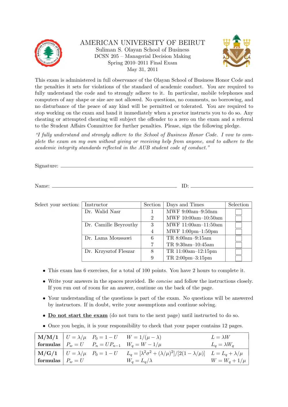
AMERICAN UNIVERSITY OF BEIRUT Suliman S. Olayan School of Business DCSN 205 – Managerial Decision Making Spring 2010–2011 Final Exam May 31, 2011 This exam is administered in full observance of the Olayan School of Business Honor Code and the penalties it sets for violations of the standard of academic conduct. You are required to fully understand the code and to strongly adhere to it. In particular, mobile telephones and computers of any shape or size are not allowed. No questions, no comments, no borrowing, and no disturbance of the peace of any kind will be permitted or tolerated. You are required to stop working on the exam and hand it immediately when a proctor instructs you to do so. Any cheating or attempted cheating will subject the offender to a zero on the exam and a referral to the Student Affairs Committee for further penalties. Please, sign the following pledge. “I fully understand and strongly adhere to the School of Business Honor Code. I vow to com- plete the exam on my own without giving or receiving help from anyone, and to adhere to the academic integrity standards reflected in the AUB student code of conduct.” Signature: Name: ID: Select your section: Instructor Section Days and Times Selection Dr. Walid Nasr 1 MWF 9:00am–9:50am 2 MWF 10:00am–10:50am Dr. Camille Beyrouthy 3 MWF 11:00am–11:50am 4 MWF 1:00pm–1:50pm Dr. Lama Moussawi 6 TR 8:00am–9:15am 7 TR 9:30am–10:45am Dr. Krzysztof Fleszar 8 TR 11:00am–12:15pm 9 TR 2:00pm–3:15pm • This exam has 6 exercises, for a total of 100 points. You have 2 hours to complete it. • Write your answers in the spaces provided. Be concise and follow the instructions closely. If you run out of room for an answer, continue on the back of the page. • Your understanding of the questions is part of the exam. No questions will be answered by instructors. If in doubt, write your assumptions and continue solving. • Do not start the exam (do not turn to the next page) until instructed to do so. • Once you begin, it is your responsibility to check that your paper contains 12 pages. 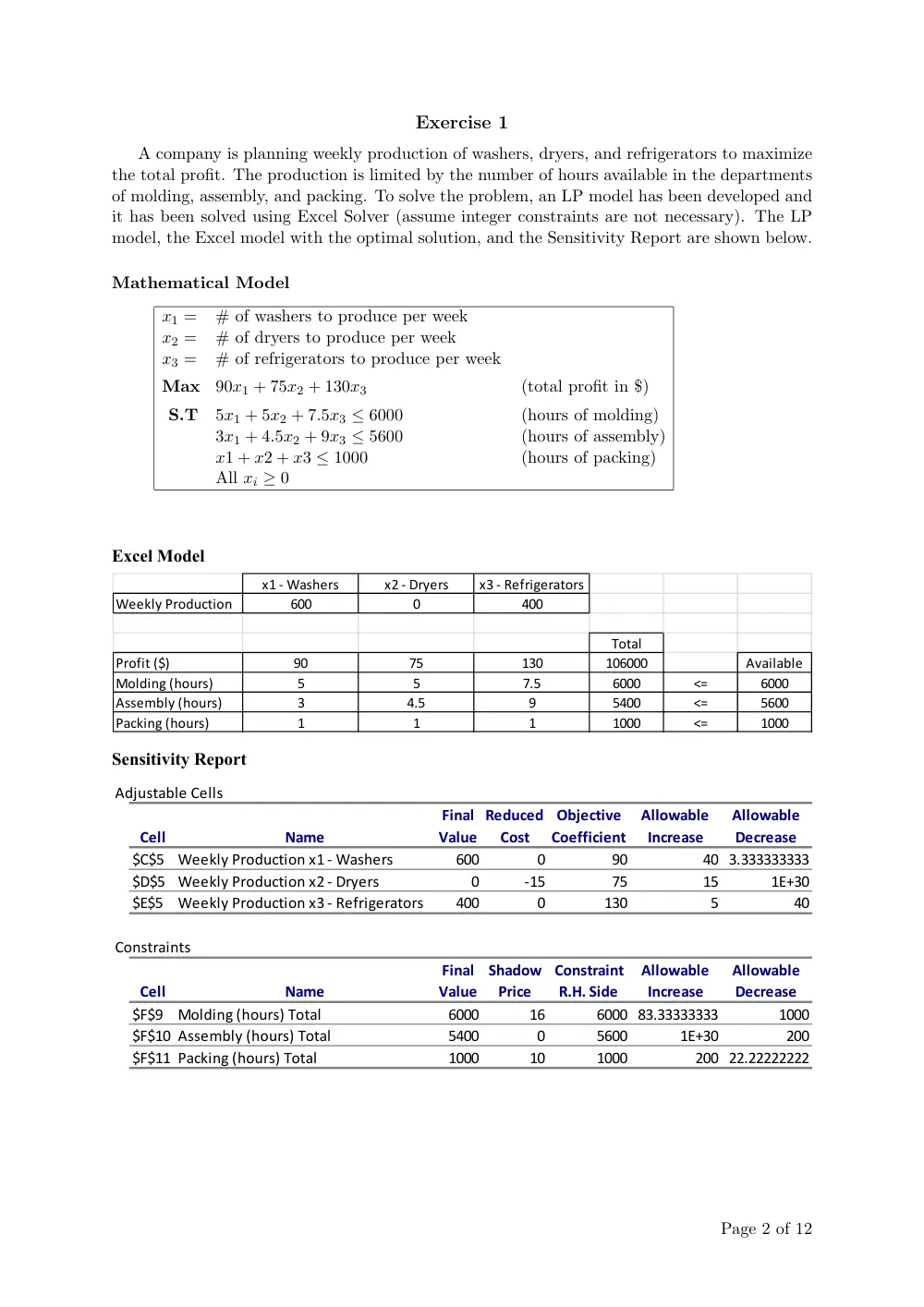M/M/1 U = λ/µ P0 = 1 − U W = 1/(µ − λ) L = λW formulas Pw = U Pn = UPn−1 Wq = W − 1/µ Lq = λWq M/G/1 U = λ/µ P0 = 1 − U Lq = [λ2σ2 + (λ/µ)2]/[2(1 − λ/µ)] L = Lq + λ/µ formulas Pw = U Wq = Lq/λ W = Wq + 1/µ Exercise 1 A company is planning weekly production of washers, dryers, and refrigerators to maximize the total profit. The production is limited by the number of hours available in the departments of molding, assembly, and packing. To solve the problem, an LP model has been developed and it has been solved using Excel Solver (assume integer constraints are not necessary). The LP model, the Excel model with the optimal solution, and the Sensitivity Report are shown below. Mathematical Model x1 = # of washers to produce per week x2 = # of dryers to produce per week x3 = # of refrigerators to produce per week Max 90x1 + 75x2 + 130x3 (total profit in $) S.T 5x1 + 5x2 + 7.5x3 ≤ 6000 (hours of molding) 3x1 + 4.5x2 + 9x3 ≤ 5600 (hours of assembly) x1 + x2 + x3 ≤ 1000 (hours of packing) All xi ≥ 0 x1 - Washers x2 - Dryers x3 - Refrigerators Weekly Production 600 0 400 Total Profit ($) 90 75 130 106000 Available Molding (hours) 5 5 7.5 6000 <= 6000 Assembly (hours) 3 4.5 9 5400 <= 5600 Packing (hours) 1 1 1 1000 <= 1000 Adjustable Cells Final Reduced Objective Allowable Allowable Cell Name Value Cost Coefficient Increase Decrease $C$5 Weekly Production x1 - Washers 600 0 90 40 3.333333333 $D$5 Weekly Production x2 - Dryers 0 -15 75 15 1E+30 $E$5 Weekly Production x3 - Refrigerators 400 0 130 5 40 Constraints Final Shadow Constraint Allowable Allowable Cell Name Value Price R.H. 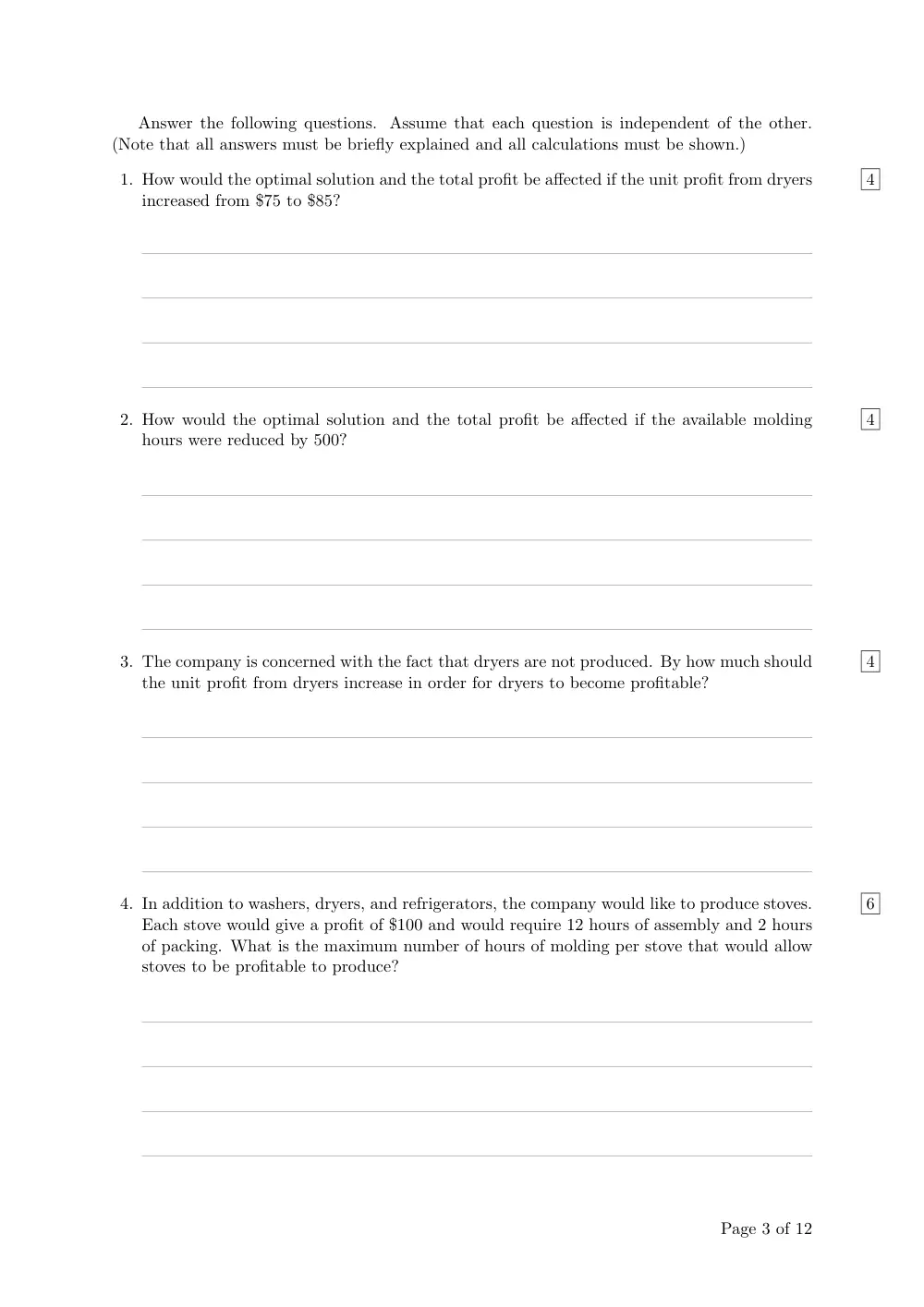Side Increase Decrease $F$9 Molding (hours) Total 6000 16 6000 83.33333333 1000 $F$10 Assembly (hours) Total 5400 0 5600 1E+30 200 $F$11 Packing (hours) Total 1000 10 1000 200 22.22222222 Excel Model Sensitivity Report Page 2 of 12 Answer the following questions. Assume that each question is independent of the other. (Note that all answers must be briefly explained and all calculations must be shown.) 1. 4 How would the optimal solution and the total profit be affected if the unit profit from dryers increased from $75 to $85? 2. 4 How would the optimal solution and the total profit be affected if the available molding hours were reduced by 500? 3. 4 The company is concerned with the fact that dryers are not produced. By how much should the unit profit from dryers increase in order for dryers to become profitable? 4. 6 In addition to washers, dryers, and refrigerators, the company would like to produce stoves. Each stove would give a profit of $100 and would require 12 hours of assembly and 2 hours of packing. What is the maximum number of hours of molding per stove that would allow stoves to be profitable to produce? 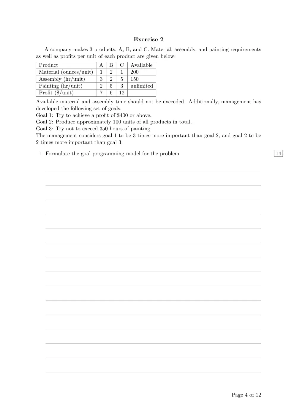Page 3 of 12 Exercise 2 A company makes 3 products, A, B, and C. Material, assembly, and painting requirements as well as profits per unit of each product are given below: Product A B C Available Material (ounces/unit) 1 2 1 200 Assembly (hr/unit) 3 2 5 150 Painting (hr/unit) 2 5 3 unlimited Profit ($/unit) 7 6 12 Available material and assembly time should not be exceeded. Additionally, management has developed the following set of goals: Goal 1: Try to achieve a profit of $400 or above. Goal 2: Produce approximately 100 units of all products in total. Goal 3: Try not to exceed 350 hours of painting. The management considers goal 1 to be 3 times more important than goal 2, and goal 2 to be 2 times more important than goal 3. 1. 14 Formulate the goal programming model for the problem. 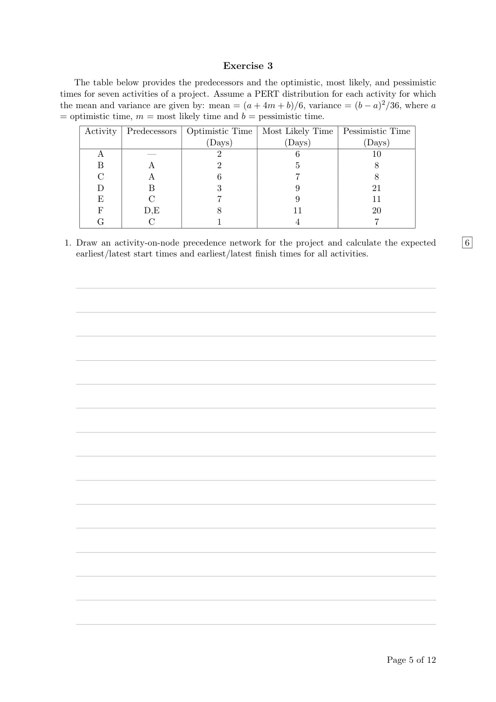Page 4 of 12 Exercise 3 The table below provides the predecessors and the optimistic, most likely, and pessimistic times for seven activities of a project. Assume a PERT distribution for each activity for which the mean and variance are given by: mean = (a + 4m + b)/6, variance = (b − a)2/36, where a = optimistic time, m = most likely time and b = pessimistic time. Activity Predecessors Optimistic Time Most Likely Time Pessimistic Time (Days) (Days) (Days) A — 2 6 10 B A 2 5 8 C A 6 7 8 D B 3 9 21 E C 7 9 11 F D,E 8 11 20 G C 1 4 7 1. 6 Draw an activity-on-node precedence network for the project and calculate the expected earliest/latest start times and earliest/latest finish times for all activities. 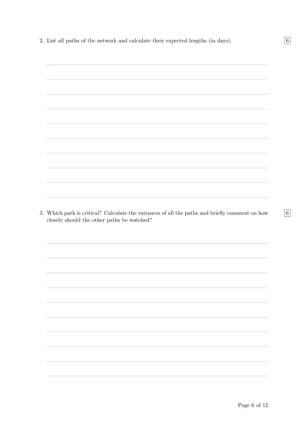Page 5 of 12 2. 6 List all paths of the network and calculate their expected lengths (in days). 3. 6 Which path is critical? Calculate the variances of all the paths and briefly comment on how closely should the other paths be watched? 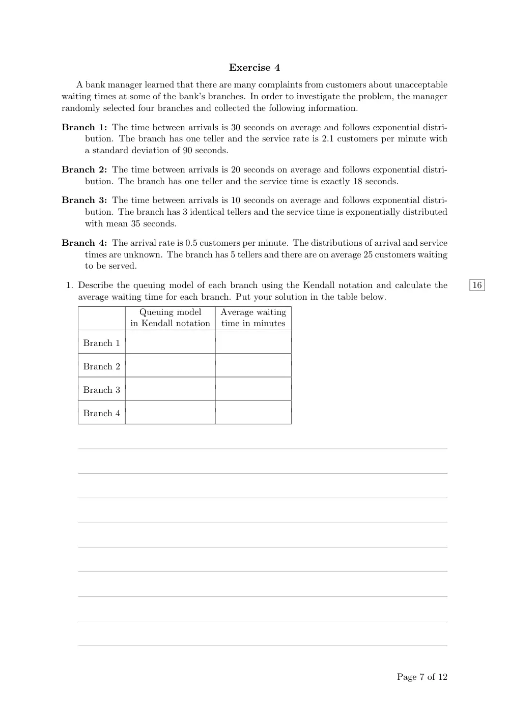Page 6 of 12 Exercise 4 A bank manager learned that there are many complaints from customers about unacceptable waiting times at some of the bank’s branches. In order to investigate the problem, the manager randomly selected four branches and collected the following information. Branch 1: The time between arrivals is 30 seconds on average and follows exponential distri- bution. The branch has one teller and the service rate is 2.1 customers per minute with a standard deviation of 90 seconds. Branch 2: The time between arrivals is 20 seconds on average and follows exponential distri- bution. The branch has one teller and the service time is exactly 18 seconds. Branch 3: The time between arrivals is 10 seconds on average and follows exponential distri- bution. The branch has 3 identical tellers and the service time is exponentially distributed with mean 35 seconds. Branch 4: The arrival rate is 0.5 customers per minute. The distributions of arrival and service times are unknown. The branch has 5 tellers and there are on average 25 customers waiting to be served. 1. 16 Describe the queuing model of each branch using the Kendall notation and calculate the average waiting time for each branch. Put your solution in the table below. 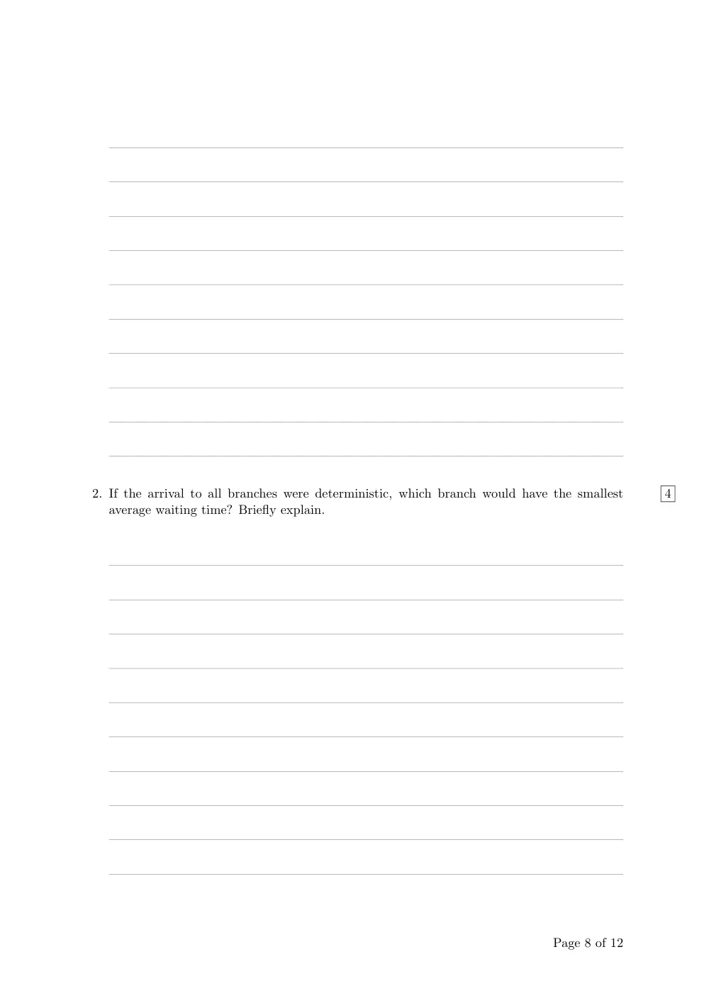Queuing model Average waiting in Kendall notation time in minutes Branch 1 Branch 2 Branch 3 Branch 4 Page 7 of 12 2. 4 If the arrival to all branches were deterministic, which branch would have the smallest average waiting time? Briefly explain. 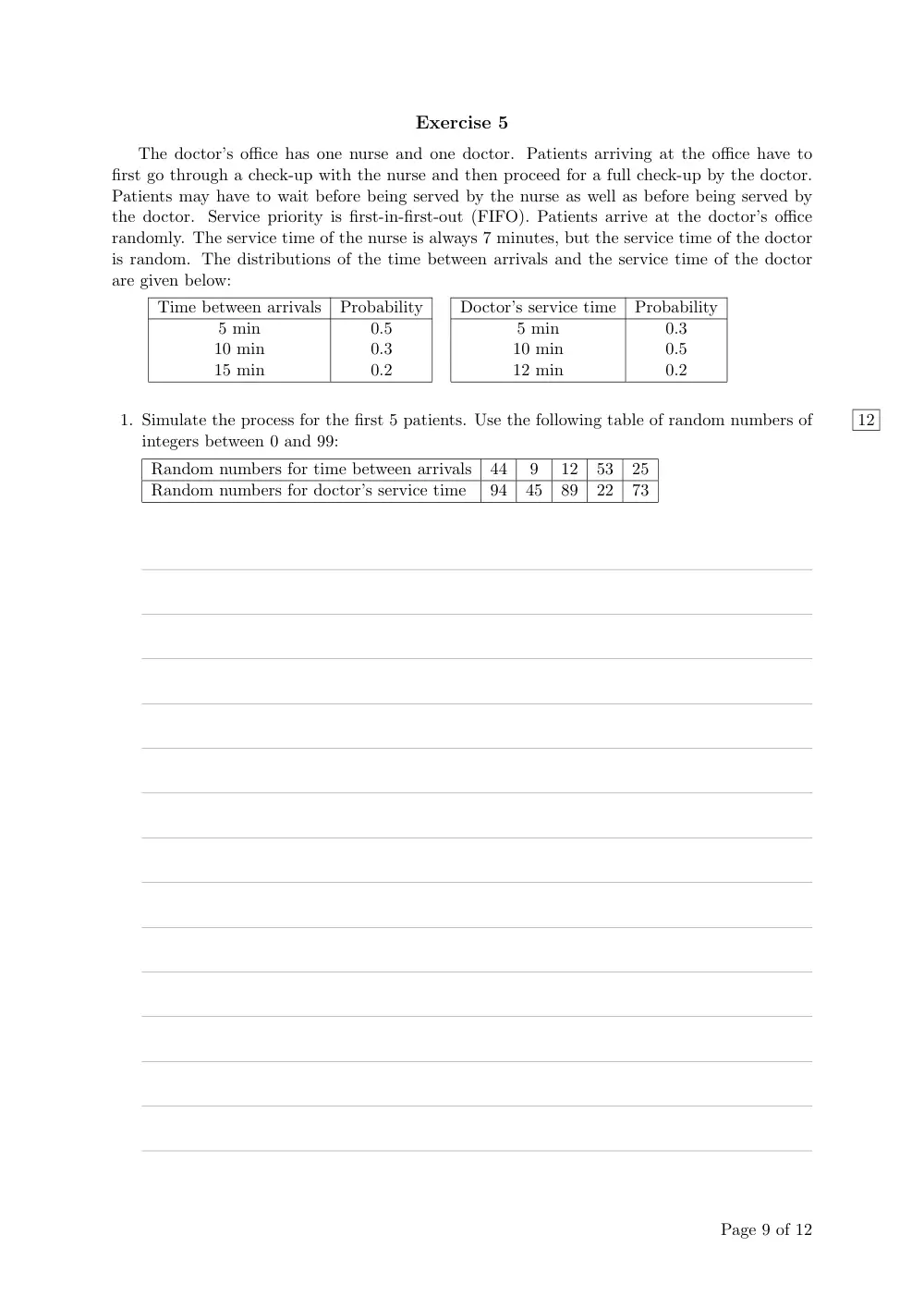Page 8 of 12 Exercise 5 The doctor’s office has one nurse and one doctor. Patients arriving at the office have to first go through a check-up with the nurse and then proceed for a full check-up by the doctor. Patients may have to wait before being served by the nurse as well as before being served by the doctor. Service priority is first-in-first-out (FIFO). Patients arrive at the doctor’s office randomly. The service time of the nurse is always 7 minutes, but the service time of the doctor is random. The distributions of the time between arrivals and the service time of the doctor are given below: Time between arrivals Probability Doctor’s service time Probability 5 min 0.5 5 min 0.3 10 min 0.3 10 min 0.5 15 min 0.2 12 min 0.2 1. 12 Simulate the process for the first 5 patients. Use the following table of random numbers of integers between 0 and 99: Random numbers for time between arrivals 44 9 12 53 25 Random numbers for doctor’s service time 94 45 89 22 73 Page 9 of 12 2. 4 Based on your simulation, how much time are the patients spending in the doctor’s office on average? Page 10 of 12 Exercise 6 Recall the decision problem of COM-TECH from Chapter 15, in which COM-TECH was considering submitting a proposal for a grant and choosing a technology upon receiving the grant. The solution was to submit the proposal and to use infrared technology if the grant is received. Note that it was still uncertain if the grant is received and if the R&D costs are high or low. The expected payoff from this solution was $13,500. The decision tree for the problem is shown below. (Note: values above events denote their probabilities; values below events and below decisions denote payoffs; values next to nodes denote expected payoffs; values on the right-hand side denote final payoffs; all payoffs are in dollars.) 0.6 High R&D Costs 16000 Microwave -60000 16000 -4000 28000 0.4 Low R&D Costs 46000 -30000 46000 0.2 High R&D Costs 0.5 5000 Receive Grant Cellular -70000 5000 3 85000 32000 -5000 29000 0.8 Low R&D Costs 35000 -40000 35000 0.1 High R&D Costs Submit Proposal -4000 Infrared -80000 -4000 -5000 13500 -4000 32000 0.9 Low R&D Costs 36000 -40000 36000 1 0.5 13500 Don't Receive Grant -5000 0 -5000 Don't Submit Proposal 0 0 0 1. 10 Perform 5 simulation runs of the COM-TECH decision problem and calculate the average payoff in dollars received by COM-TECH in your simulation. In each simulation run, generate two random events: one if the grant is received or not and the other if the R&D costs are high or low. Use the following table of random numbers between 0 and 99: Random numbers for receiving the grant or not 34 45 89 32 73 Random numbers for high or low R&D costs 4 9 32 73 25 Page 11 of 12 2. 4 Compare the average payoff from your simulation with the expected payoff from the decision tree. Briefly explain the cause of the difference. Page 12 of 12