ECON 211 Problems For Chapters 2, Spring 2008

ECONOMICS 211: INTRODUCTORY MICROECONOMIC THEORY SPRING 2005 American University of Beirut Department of Economics Table of Contents CHAPTER 2: THE ECONOMIC PROBLEM: SCARCITY AND CHOICE .....................1 Problem 1: Production Possibility Frontier I ...................................................................1 Problem 2: Production Possibility Frontier II..................................................................3 Problem 3: Absolute and Comparative Cost Advantage .................................................4 CHAPTER 3: DEMAND, SUPPLY AND MARKET EQUILIBRIUM.............................6 Problem 1: Demand, Supply, and Price ...........................................................................6 Problem 2: Demand, Supply, and Price ...........................................................................7 Problem 3: Demand, Supply, and Price ...........................................................................8 Problem 4: Demand, Supply, and Price ...........................................................................9 Problem 5: Demand, Supply, and Price .........................................................................11 Problem 6: Demand, Supply, and Price .........................................................................12 Problem 7: Demand, Supply, and Price .........................................................................13 Problem 8: Demand, Supply, and Price .........................................................................14 CHAPTER 4: DEMAND AND SUPPLY APPLICATIONS AND ELASTICITY..........15 Problem 1: Elasticity.....................................................................................................15 Problem 2: Income Elasticity of Demand......................................................................19 Problem 3: The Laffer Curve .........................................................................................20 CHAPTER 5: HOUSEHOLD BEHAVIOR AND CONSUMER CHOICE.....................21 Problem 1: Total Utility vs. Marginal Utility and Demand Curve ................................21 Problem 2: Aggregate Demand......................................................................................23 Problem 3: Income and Substitution Effect ...................................................................24 Problem 4: Income and Substitution Effect ...................................................................25 CHAPTERS 6/7: THE PRODUCTION PROCESS: THE BEHAVIOR OF PROFIT MAXIMIZING FIRMS/SHORT RUN COSTS AND OUTPUT DECISIONS................26 Problem 1: Profit Maximization ....................................................................................26 Problem 2: Total Product, Average Product, Marginal Product....................................27 Problem 3: Total Costs, Average Total Costs, Average Variable Cost, Marginal Cost 28 Problem 4: Output Decisions in the Short-Run and Market Entry................................29 CHAPTER 8: LONG RUN COSTS AND OUTPUT DECISIONS..................................31 Problem 1: Cost Curves of Single-Product Firm ...........................................................31 Problem 2: Long-Run Cost Minimization.....................................................................32 CHAPTER 9: INPUT DEMAND: LABOR MARKETS..................................................33 Problem 1: Demand for Factor Labor ............................................................................33 Problem 2: Income and Substitution Effect in the Labor Market..................................34 CHAPTER 12: MONOPOLY AND ANTITRUST POLICY ...........................................35 Problem 1: Monopoly, Perfect Competition, and Cartel...............................................35 CHAPTER 13: MONOPOLISTIC COMPETITION AND OLIGOPOLY.......................38 Problem 1: Perfect Competition, Monopolistic Competition, and Monopoly...............38 Problem Set 2: Game Theory.........................................................................................43 1 CHAPTER 2: THE ECONOMIC PROBLEM: SCARCITY AND CHOICE Problem 1: Production Possibility Frontier I A B C D E F G Frisbees 0 45 80 110 130 145 150 Boomerangs 200 190 170 140 100 50 0 20 40 80 100 120 140 160 180 200 40 60 60 80 100 120 140 200 Boomerangs Frisbees 160 180 20 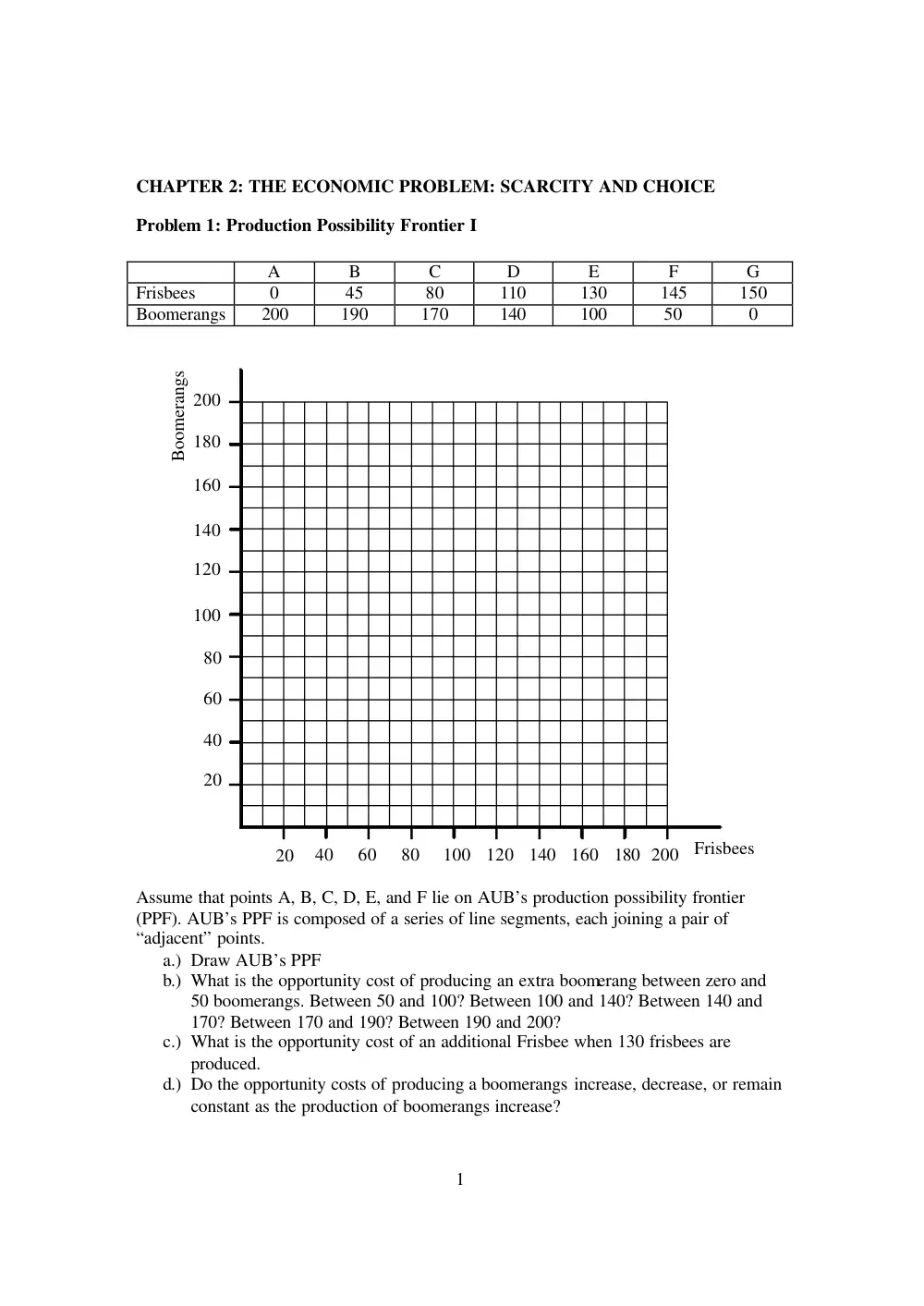Assume that points A, B, C, D, E, and F lie on AUB’s production possibility frontier (PPF). AUB’s PPF is composed of a series of line segments, each joining a pair of “adjacent” points. a.) Draw AUB’s PPF b.) What is the opportunity cost of producing an extra boomerang between zero and 50 boomerangs. Between 50 and 100? Between 100 and 140? Between 140 and 170? Between 170 and 190? Between 190 and 200? c.) What is the opportunity cost of an additional Frisbee when 130 frisbees are produced. d.) Do the opportunity costs of producing a boomerangs increase, decrease, or remain constant as the production of boomerangs increase? 2 Problem 1: Production Possibility Frontier I (Continued) e.) Indicate which areas of the graph correspond to a. infeasible production points b. production points where there is unemployment c. efficient production points f. Suppose that the AUB economy is producing at point D. One day President Waterbury suggests that fewer resources be used to produce Frisbees and more for boomerangs. As a result, the AUB community moves to point C, which president Waterbury claims is more efficient? Why is point C more efficient? g. How would AUB’s PPF be altered by an improvement in the technology of producing boomerangs? h. President Waterbury annexes a nearby college which has the same technology as AUB but only half the resources. This takeover creates what President Waterbury calls “Greater AUB.” How does Greater AUB’s PPF compare to the PPF of part a.) above? 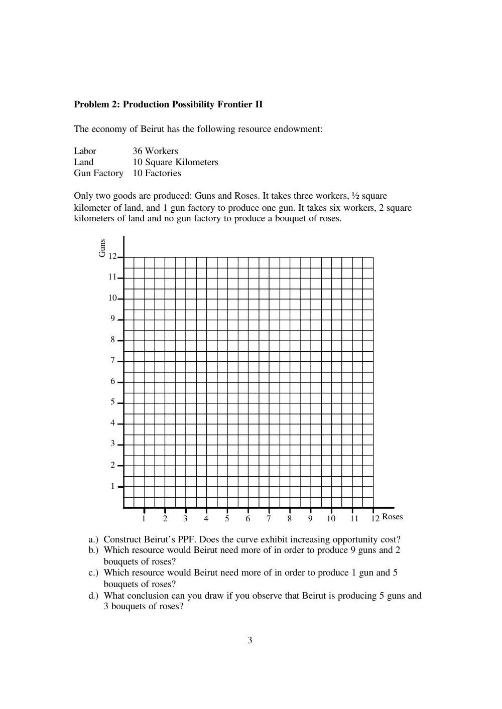3 Problem 2: Production Possibility Frontier II The economy of Beirut has the following resource endowment: Labor 36 Workers Land 10 Square Kilometers Gun Factory 10 Factories Only two goods are produced: Guns and Roses. It takes three workers, ½ square kilometer of land, and 1 gun factory to produce one gun. It takes six workers, 2 square kilometers of land and no gun factory to produce a bouquet of roses. 1 2 3 4 5 6 7 8 9 10 11 12 1 2 3 4 5 6 7 10 11 12 9 8 Roses Guns a.) Construct Beirut’s PPF. Does the curve exhibit increasing opportunity cost? b.) Which resource would Beirut need more of in order to produce 9 guns and 2 bouquets of roses? c.) Which resource would Beirut need more of in order to produce 1 gun and 5 bouquets of roses? d.) What conclusion can you draw if you observe that Beirut is producing 5 guns and 3 bouquets of roses? 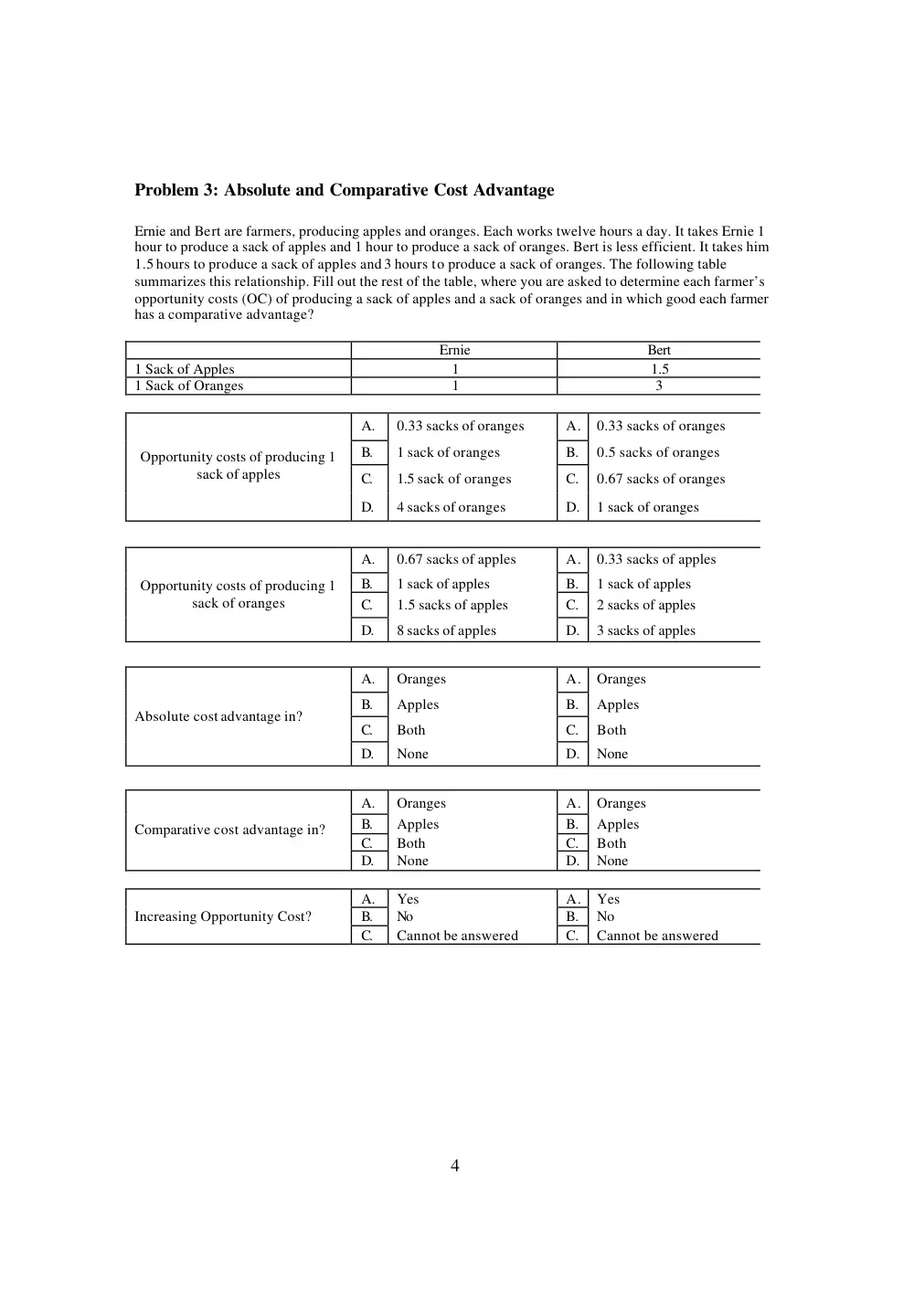4 Problem 3: Absolute and Comparative Cost Advantage Ernie and Bert are farmers, producing apples and oranges. Each works twelve hours a day. It takes Ernie 1 hour to produce a sack of apples and 1 hour to produce a sack of oranges. Bert is less efficient. It takes him 1.5 hours to produce a sack of apples and 3 hours to produce a sack of oranges. The following table summarizes this relationship. Fill out the rest of the table, where you are asked to determine each farmer’s opportunity costs (OC) of producing a sack of apples and a sack of oranges and in which good each farmer has a comparative advantage? Ernie Bert 1 Sack of Apples 1 1.5 1 Sack of Oranges 1 3 A. 0.33 sacks of oranges A. 0.33 sacks of oranges B. 1 sack of oranges B. 0.5 sacks of oranges C. 1.5 sack of oranges C. 0.67 sacks of oranges Opportunity costs of producing 1 sack of apples D. 4 sacks of oranges D. 1 sack of oranges A. 0.67 sacks of apples A. 0.33 sacks of apples B. 1 sack of apples B. 1 sack of apples C. 1.5 sacks of apples C. 2 sacks of apples Opportunity costs of producing 1 sack of oranges D. 8 sacks of apples D. 3 sacks of apples A. Oranges A. Oranges B. Apples B. Apples C. Both C. Both Absolute cost advantage in? D. None D. None A. Oranges A. Oranges B. Apples B. Apples C. Both C. Both Comparative cost advantage in? D. None D. None A. Yes A. Yes B. No B. No Increasing Opportunity Cost? C. Cannot be answered C. 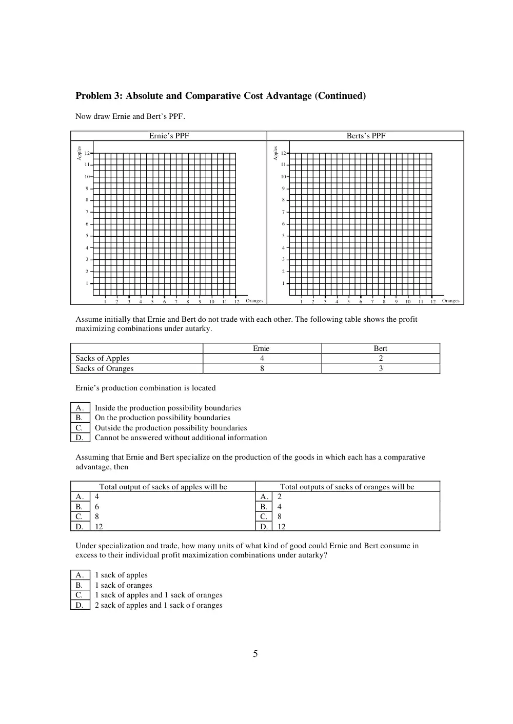Cannot be answered 5 Problem 3: Absolute and Comparative Cost Advantage (Continued) Now draw Ernie and Bert’s PPF. Ernie’s PPF Berts’s PPF 1 2 3 4 5 6 7 8 9 10 11 12 1 2 3 4 5 6 7 10 11 12 9 8 Apples Oranges 1 2 3 4 5 6 7 8 9 10 11 12 1 2 3 4 5 6 7 10 11 12 9 8 Apples Oranges Assume initially that Ernie and Bert do not trade with each other. The following table shows the profit maximizing combinations under autarky. Ernie Bert Sacks of Apples 4 2 Sacks of Oranges 8 3 Ernie’s production combination is located A. Inside the production possibility boundaries B. On the production possibility boundaries C. Outside the production possibility boundaries D. Cannot be answered without additional information Assuming that Ernie and Bert specialize on the production of the goods in which each has a comparative advantage, then Total output of sacks of apples will be Total outputs of sacks of oranges will be A. 4 A. 2 B. 6 B. 4 C. 8 C. 8 D. 12 D. 12 Under specialization and trade, how many units of what kind of good could Ernie and Bert consume in excess to their individual profit maximization combinations under autarky? A. 1 sack of apples B. 1 sack of oranges C. 1 sack of apples and 1 sack of oranges D. 2 sack of apples and 1 sack o f oranges 6 CHAPTER 3: DEMAND, SUPPLY AND MARKET EQUILIBRIUM Problem 1: Demand, Supply, and Price How does each of the following events affect the market for chickens? For each, discuss which curve has shifted. Holding everything else constant, discuss also the resulting change in equilibrium price and quantity a. A severe winter reduces the cattle population. b. The price of poultry feed decreases. c. Chicken is found to be a good source of a newly discovered nutrient. d. A cheaper method is found for preventing chicken cannibalism. e. There is a rapid increase in the human population. f. There is a recession and consumers expect significant lower incomes. g. Betty Crocker markets a quicker, cheaper stuffing mix. 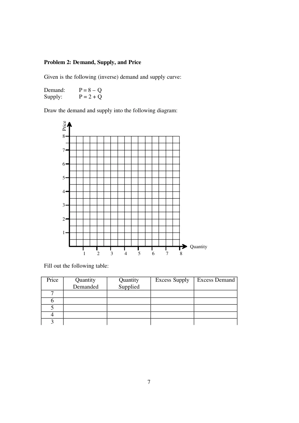7 Problem 2: Demand, Supply, and Price Given is the following (inverse) demand and supply curve: Demand: P = 8 – Q Supply: P = 2 + Q Draw the demand and supply into the following diagram: 1 2 3 4 5 6 7 8 1 2 3 4 5 6 7 8 Quantity Price Fill out the following table: Price Quantity Demanded Quantity Supplied Excess Supply Excess Demand 7 6 5 4 3 8 Problem 3: Demand, Supply, and Price 1 2 3 4 5 6 7 8 9 10 11 12 1 2 3 4 5 6 7 10 11 12 9 8 Quantity Price 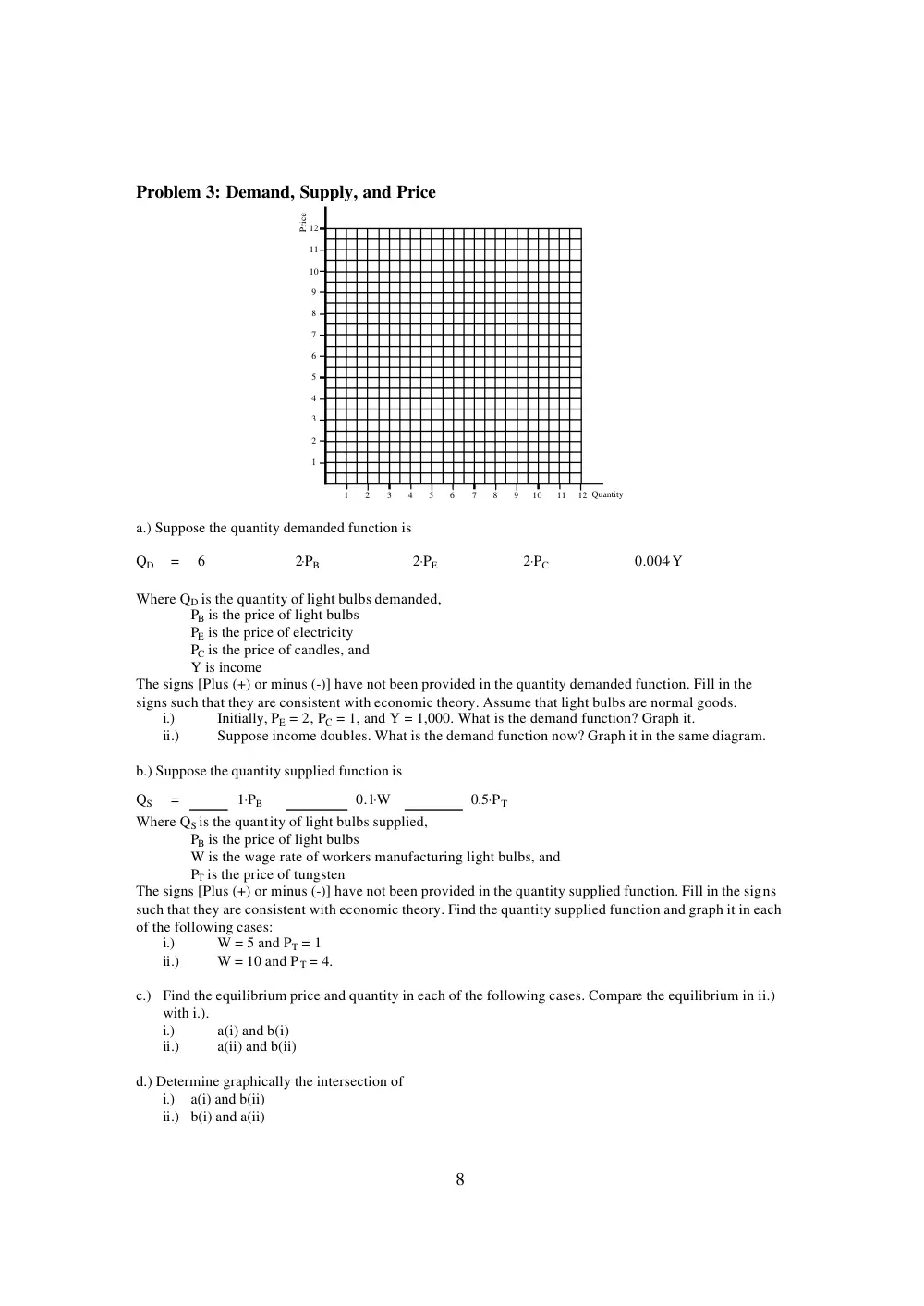a.) Suppose the quantity demanded function is QD = 6 2⋅PB 2⋅PE 2⋅PC 0.004⋅Y Where QD is the quantity of light bulbs demanded, PB is the price of light bulbs PE is the price of electricity PC is the price of candles, and Y is income The signs [Plus (+) or minus (-)] have not been provided in the quantity demanded function. Fill in the signs such that they are consistent with economic theory. Assume that light bulbs are normal goods. i.) Initially, PE = 2, PC = 1, and Y = 1,000. What is the demand function? Graph it. ii.) Suppose income doubles. What is the demand function now? Graph it in the same diagram. b.) Suppose the quantity supplied function is Where QS is the quantity of light bulbs supplied, PB is the price of light bulbs W is the wage rate of workers manufacturing light bulbs, and PT is the price of tungsten The signs [Plus (+) or minus (-)] have not been provided in the quantity supplied function. Fill in the signs such that they are consistent with economic theory. Find the quantity supplied function and graph it in each of the following cases: i.) W = 5 and PT = 1 ii.) W = 10 and PT = 4. c.) Find the equilibrium price and quantity in each of the following cases. Compare the equilibrium in ii.) with i.). i.) a(i) and b(i) ii.) a(ii) and b(ii) d.) Determine graphically the intersection of i.) a(i) and b(ii) ii.) b(i) and a(ii) QS = 1⋅PB 0.1⋅W 0.5⋅PT 9 Problem 4: Demand, Supply, and Price 1. Given is the following demand curve (D): D: P = 8-Q Assume two different supply curves, S1 and S2: S1: P = Q S2: P = 4 Denote the intersection between demand and the two supply curves as point A. Now assume that government introduces a sales tax (T) of T = 2. Discuss the effects on market price, new quantity actually bought, and welfare in dependence of the different supply curves. Using the following diagram may help. 1 2 3 4 5 6 7 1 2 3 4 5 6 7 8 Quantity 8 Price 10 Problem 4: Demand, Supply, and Price (Continued) 2. Given is the following supply curve (S): S: P = 1 + Q Assume two different demand curves, D1 and D2: D1: Q = 4 S2: P = 7 - Q Denote the intersection between supply and the two demand curves as point A. Now assume that government introduces a sales tax (T) of T = 2. Discuss the effects on market price, quantity actually bought, and welfare in dependence of the different demand curves. Using the following diagram may help. 1 2 3 4 5 6 7 1 2 3 4 5 6 7 8 Quantity 8 Price 11 Problem 5: Demand, Supply, and Price Consider the following demand and supply equations for bread in Lebanon. QD is quantity of bread demanded by consumers (in millions of kilos per month), QS is quantity of bread supplied (in millions of kilos per month), PB is the market price for kilo of bread (in 1,000s of Lebanese Liras), and I is monthly income (in 1,000s of Lebanese Liras). QD = 10 - 1⋅PB + 1/300⋅I QS = 2⋅PB – 6 a. If average income per month is I = 600, what is the equilibrium quantity and price? Illustrate this on the graph below. Please conduct a welfare analysis of the market. 1 2 3 4 5 6 7 8 9 10 11 12 13 14 15 16 1 2 3 4 5 6 7 8 9 10 11 12 13 14 15 16 Quantity P b. The government finds that the price of bread is too high and decides to impose a price ceiling of LL 5,000 per kilo. What are the new quantities demanded and supplied in the market? What is the amount of the surplus or shortage? What is the quantity of bread exchanged in the market? How does welfare change? c. After imposing the price ceiling, the government conducts a survey and finds that most consumers who want bread are able to obtain the quantity they want. Suggest possible explanations for this finding. Think outside the box. d. The Lebanese government decides to abandon price controls in favor of a per unit subsidy (S) of S = 1,500 per kilo of bread produced. Illustrate graphically and compare the effects of this policy from a welfare perspective to the situation in a.). How much does the subsidy program cost government? e. Going back to ques tion a., assume Prime Minister Hariri sells one of his mountains and islands and passes on the revenues as a tax break to the Lebanese people, so that disposable income goes up from I = 600 to INew =1,500. Holding everything else constant, how does this change equilibrium quantity, price, and welfare? Illustrate your results again graphically. 12 Problem 6: Demand, Supply, and Price Draw all relevant graphs into the following diagram. 1 2 3 4 5 6 7 8 1 2 3 4 5 6 7 8 Quantity Price a. Assume the initial demand (D1) and supply (S1) for coffee is D1: P = 6–0.5Q and S1: P=Q, respectively. What are equilibrium price and quantity? Denote this equilibrium “Point A.” b. As a result of a tropical storm in Banana Republic, which destroyed a substantial amount of the coffee plantation, the new supply curve (S2) is S2: P = 3+Q. What are the new equilibrium price and quantity? Denote this equilibrium “Point B.” c. Now assume that in addition to the reduction of supply, people anticipate a shortage of coffee and begin hoarding coffee. The new demand curve (D2) is D2: P=7.5-0.5Q. What are the new equilibrium price and quantity? Denote this equilibrium “Point C.” d. Identify all shifts and movements of demand and supply when moving from “A” over “B” to “C.” e. Comparing “Point A” and “Point C,” why did the decrease in supply and increase in demand not cancel out in terms of quantity demanded and quantity supplied? f. Calculate the point elasticity of demand and supply in point A, B, and C. g. Since the price of coffee has increased dramatically, the government of Banana Republic decides to impose a maximum price on coffee of PMax=4. Discuss the results. h. As a result of the maximum price, many have lost their job. More and more go on the streets and demonstrate for a policy change. Eventually, a new government takes over and promises to create new jobs. As a first step, the new government abandons the price ceiling on coffee and replaces it by a minimum price of PMin=7 so that it “pays again” to produce coffee and to hire people. How do you evaluate this new policy? 13 Problem 7: Demand, Supply, and Price Given is the following import demand curve (D): D: P = 8 - Q Assume three different import supply curves, S1, S2, and S3. S1: P = 4 S2: P = Q S3: Q = 4 1.What are the quantities imported given S1, S2, and S3? 2.What are the market prices given S1, S2, and S3? 3.Assume government introduces an import tariff (T) of T=2. What are the new import- supply curves given S1, S2, and S3? 4.What are the new quantities imported? 5.What are the new market prices? 6.What are total tariff revenues? 7.Which percentage of the tariff is passed on to the consumers? S1 S2 S3 1. Quantity imported 2. Market price 3. New supply curves 4. New quantities imported 5. New market prices 6. Tariff revenues 7. Percentage passed on to consumers 1 2 3 4 5 6 7 1 2 3 4 5 6 7 8 Quantity 8 Price 14 Problem 8: Demand, Supply, and Price Assume the following demand and supply curves for grain in the European Union (EU). The supply in the European Union is made up of domestic supply by European producers (SEU) and import supply by World producers (SWorld). DEU: P = 8-Q SEU: P = 2+Q SWorld: P = 3 1. What is the equilibrium price and quantity? How much is domestically produced and how much is imported? 2. Since European Farmers can barely compete with World imports, European farmers lobby successfully for an import tariff of T = 4 and a price floor for grain of PFloor = 6. What is the new equilibrium price and quantity? How much is domestically produced and how much is imported? 3. The EU is increasingly confronted with non-sellable mountains of grain. So the EU commission for smart economic development policy decides to ship European excess supply to Africa for free. Africa’s demand and supply curve for grain are: DAfr.: P = 6-Q SAfr.: P = 2+Q a. What is the equilibrium price and quantity in Africa? b. What is Africa’s new supply curve after the EU sent its benevolent gift? c. How does the grain gift benefit African grain output and African grain prices? d. Who wins and who loses from the EU’s policy in Europe and in Africa? EU Market Africa’s Market 1 2 3 4 5 6 7 8 1 2 3 4 5 6 7 8 P Q 1 2 3 4 5 6 7 8 1 2 3 4 5 6 7 8 P Q 15 CHAPTER 4: DEMAND AND SUPPLY APPLICATIONS AND ELASTICITY Problem 1: Elasticity 1. Draw the following three inverse demand curves into the diagram below: D1: P = 8 – Q D2: P = 8 – 2Q D3: P = 8 – 4 Q Calculate for all three demand curves the point elasticity of demand for P = 4. 1 2 3 4 5 6 7 1 2 3 4 5 6 7 8 Quantity 8 Price 16 Problem 1: Elasticity (Continued) 2. Draw the following two inverse demand curves into the diagram below: D1: P = 6 – Q D2: P = 5 – 0.5 Q 1 2 3 4 5 6 7 1 2 3 4 5 6 7 8 Quantity 8 Price Calculate for all two demand curves the point elasticity of demand at P = 4. 17 Problem 1: Elasticity (Continued) 3. Draw the following two demand curves into the diagram below: D1: P = 4 – Q D2: P = 8 – 2Q 1 2 3 4 5 6 7 1 2 3 4 5 6 7 8 Quantity 8 Price Calculate for all two demand curves the point elasticity of demand for Q = 2. 18 Problem 1: Elasticity (Continue d) 4. Draw the following two demand curves into the diagram below: D1: P = 4 – Q D2: P = 8 – Q 1 2 3 4 5 6 7 1 2 3 4 5 6 7 8 Quantity 8 Price Calculate for all two demand curves the point elasticity of demand for Q = 2 and then for P = 2. 19 Problem 2: Income Elasticity of Demand Point A Point B Point C Point D Income 1 3 5 7 Demand 1 3 3 1 Draw Point A, B, C, and D in the following diagram and connect them by straight lines assuming that those lines represent demand functions in dependence of income. 1 2 3 4 5 6 7 1 2 3 4 5 6 7 8 Income (Y) 8 Demand (Q) 1. Find the demand function (D) of income for D(A � B), D(B �C), and D(C � D). 2. What’s the income elasticity of demand at the following levels of income (Y): Y = 2, Y = 4, and Y = 6? 20 Problem 3: The Laffer Curve The Laffer curve depicts the relationship between taxes and tax revenues as an inverse U. Many politicians all over the world have already made some rather frustrating acquaintance with Mr. Laffer’s curve. For example, many governments raised taxes on cigarettes hoping to fill their budget deficits only to find out that tax revenues eventually decreased. Assume that the demand curve for cigarettes in dependence of the tax rate (T) is Demand: T = 5 – Q Complete the following table and calculate the different tax revenues (TR) for the different Ts as well as the corresponding point elasticities. Ts 0 0.5 1 1.5 2 2.5 3 3.5 4 4.5 5 TR e Assume you are a policy consultant to a government, which considers increasing the tax rate on cigarettes from T = 2 to T = 3. Would you support or oppose the government’s plans? Discuss your result. 1 2 3 4 5 6 1 2 3 4 5 6 Quantity Price 1 2 3 4 5 6 1 2 3 4 5 6 Quantity TR 21 CHAPTER 5: HOUSEHOLD BEHAVIOR AND CONSUMER CHOICE Problem 1: Total Utility vs. Marginal Utility and Demand Curve As school increasingly stresses you out, you decide to take a couple of days off and to head for the beach for a real sun and fun deal. Since you want to look great at the beach and at the night clubs that you plan to visit extensively, you decide to buy some new outfits for the beach (B) and some elegant clothes (E) for the nightlife. 1. Draw the total and marginal utility functions for B and E. 2. If you have a budget of USD 160 and an item of each beach and elegant wear costs USD 20, how many items of beach wear and elegant wear will you buy? Why would you not buy five items of elegant wear and three items of beach wear? How big is your consumer surplus for beach and elegant wear, respectively? 3. If you have a budget of USD 160 and an item of beach wear costs USD 20 and an item of elegant wear costs USD 40, how many items of beach wear and how many items of elegant wear would you buy? Why would you not buy three items of elegant wear and two items of beach wear? How big is your consumer surplus for beach and elegant wear, respectively? 4. Locate the price-demand combination for elegant wear in a diagram. Estimate the shape of the demand curve for elegant wear for all prices. 5. Now assume that you and two of your best friends, who have exactly the same budget and preferences like you, join you to the beach. Locate the combined price-demand combinations of you three for elegant wear in a diagram. Estimate the shape of the aggregate demand curve for elegant wear for all prices. Sketch the area that represents consumer surplus. Beach Wear (B) Elegant Wear (E) Qty. Total Utility (B) Marginal Utility (B) PB MU B ) ( Total Utility (E) Marginal Utility (E) PE MU E ) ( 1 250 350 2 450 550 3 600 700 4 700 800 5 775 875 6 800 900 22 Problem 1: Total Utility versus Marginal Utility and Demand Curve (Contd.) to Q1: 1 2 3 4 5 6 7 8 9 10 1 2 3 4 5 6 7 8 9 10 Total Utility Q 1 2 3 4 5 6 7 8 9 10 1 2 3 4 5 6 7 8 9 10 Marginal Utility Q to Q4 and Q5: 1 2 3 4 1 2 3 4 5 6 Q 1 2 3 4 3 6 9 12 15 18 Q Individual Aggregate The numbers on the y-Axis are in 100s 23 Problem 2: Aggregate Demand Quantity Price 1 2 3 4 5 6 7 8 1 2 3 4 1 2 3 4 5 6 7 8 1 2 3 4 5 6 7 8 9 10 Price Quantity Form with the three individual demand curves from the left panel the aggregate demand curve in the right panel. 24 Problem 3: Income and Substitution Effect a.) Assume you have a budget (B) of B = 100 that you spend on chocolate bars (C) and ice cream (I). Initially, the prices for chocolate bars and ice cream are PC = 2 and PI = 2. Draw the budget line and determine the consumption plan. Now assume that – holding everything else constant - the price for chocolate bars falls to PCNew = 1. Draw the new budget line, and determine the new optimum consumption plan, as well as the income and substitution effect. b.) Now repeat the same exercise, assuming that the initial prices were PI =2 and PC =1, respectively, and PC increased to PC New = 2. 10 20 30 40 50 60 70 80 90 100 10 20 30 40 50 60 70 80 90 100 C I 10 20 30 40 50 60 70 80 90 100 10 20 30 40 50 60 70 80 90 100 C I 25 Problem 4: Income and Substitution Effect Given is the utility function X Y 2 U ⋅ = . Your budget (B) is B=$6. The prices for x and y are px=1 and py=2, respectively. a.) Draw the budget line into the diagram below. b.) How many x and y do you buy in order to maximize your utility? How big is your total utility? Draw the indifference curve into the diagram below. c.) Now assume that the price for y falls from p y = 2 to py =1. Draw the new budget line into the diagram below. d.) How many x and y do you buy now in order to maximize your utility? How big is your new total utility? Draw the new indifference curve into the diagram below. e.) Estimate the income and substitution effect graphically? f.) Difficult: Determine the income and substitution effect mathematically. Good Luck! 1 2 3 4 5 6 7 8 9 10 11 12 1 2 3 4 5 6 7 10 11 12 9 8 X Y 26 CHAPTERS 6/7: THE PRODUCTION PROCESS: THE BEHAVIOR OF PROFIT MAXIMIZING FIRMS/SHORT RUN COSTS AND OUTPUT DECISIONS Problem 1: Profit Maximization TR TC Q TR TQ Q Profit A B The total cost function is: TC = 10+5q-3q2+1/3q3 The total revenue function is: TR = 2.25 q Determine the quantities associated with point A, E and F as well as the associated profits (Round to first decimal). 27 Problem 2: Total Product, Average Product, Marginal Product Given is the following total product curve. Derive the marginal and average product curve graphically. TP Q Q Total Product Marginal Product Average Product 28 Problem 3: Total Costs, Average Total Costs, Average Variable Cost, Marginal Cost Given is the following total cost curve. Derive the marginal, total average, and variable average cost curve graphically. Q TC CFix Q Costs Costs 29 Problem 4: Output Decisions in the Short-Run and Market Entry Assume a market with two firms that compete perfectly. The total cost function of the typical firm is 1 2 2 + + = Q Q TC The (inverse) demand function is Q P = 12 − 1. The following questions refer to the short run equilibrium: a.) What is the supply curve of one firm, QSi? b.) What is the (horizontally added) supply curve of the two firms in the market, QS? c.) What is the equilibrium price and quantity, P* and Q*, respectively? d.) Determine the following: a. Producer surplus of the individual firm b. Producer surplus of the industry c. Profit of the individual firm d. Industry profit e. Consumer surplus f. Welfare g. (Point) price elasticity of demand in the equilibrium price 2. The following questions refer to the introduction of a tax: a.) Assume now that government imposes a tax of T= 2. Determine the following: a. New aggregate supply curve of the two firms b. Equilibrium price and quantity c. Total tax revenues d. Producer surplus of the individual firm e. Producer surplus of the industry f. Tax burden that producers roll over to consumers (in percent) g. Profit of the individual firm h. Industry profit i. Consumer surplus j. Welfare k. Dead weight loss l. (Point) price elasticity of demand in the (new) equilibrium price 30 3. The following questions refer to the long run equilibrium? a.) How many firms will be there in the long run? b.) Determine the following: a. Producer surplus of the individual firm b. Producer surplus of the industry c. Profit of the individual firm d. Industry profit e. Consumer surplus f. Welfare g. (Point) price elasticity of demand in the equilibrium price 1 2 3 4 5 6 7 8 9 10 11 12 1 2 3 4 5 6 7 10 11 12 9 8 Quantity Price 1 2 3 4 5 6 7 8 9 10 11 12 1 2 3 4 5 6 7 10 11 12 9 8 Quantity Price 31 CHAPTER 8: LONG RUN COSTS AND OUTPUT DECISIONS Problem 1: Cost Curves of Single-Product Firm Below you see stylized cost curves. 1. What is the (vertical) value of Point 1? a. 100 b. 150 c. 200 d. 300 e. 450 2. What is the (vertical) value of Point 2? a. 1 b. 2 c. 3 d. 4 e. 5 3. What is the (vertical) value of Point 3? a. 24 b. 26 c. 28 d. 30 e. 32 4. What is the (horizontal) value of Point 4? a. 2 b. 2.5 c. 3 d. 3.5 e. 4 5. What is the average total cost associated with the (horizontal) value of Point 4? a. 16 b. 18 c. 20 d. 22 e. 24 6. What is the average variable cost associated with the (horizontal) value of point 4? a. 6 b. 8 c. 10 d. 12 e. Cannot be answered without additional information. 32 Problem 2: Long-Run Cost Minimization Given is the following production function of a firm: L K Q ⋅ = 2 , where Q=Output, K=Capital, and L=Labor. The price for capital is pK = 4 and the price for labor pL = 2 . The company wants to produce Q=64 at minimum costs. 1 2 3 4 5 6 7 8 9 10 1 2 3 4 5 6 7 8 9 10 Capital Labor 1. What is the cost minimizing relationship between K and L? A. 0.5K=L B. 0.5L=K C. K=L D. K=4L 2. In the optimum, the firm will use A. K=L=4 B. K=2; L=16 C. K=3, L=3 D. None of the above answers is correct 3. What are the total costs of the cost minimizing output? A. 22 B. 40 C. 18 D. 24 4. Referring to the diagram with capital on the y-axis and labor on the x-axis, what is the marginal rate of transformation at L=1? A. -2 B. -4 C. -6 D. -8 5. Assume that factor labor received training, increasing its productivity such that the production function becomes K 2 L2 QNew ⋅ = . Holding everything else constant, what is the new cost- minimizing relationship between K and L? A. Eight times as many L as K B. Twice as many