EECE 231 Lab 1024, Fall 2017

Circuits and Electronics Lab (ECE 312L): Experiment number 4: RC circuits Names: Taha Dani and Abdul Aziz M.Abi Haydar ID numbers: 201700147 and 201703752 respectively Email: tmd11@mail.aub.edu and ama204@mail.aub.edu Section number: 3 Group number: 9 Date: 12/10/2017 Table of Contents: I. OBJECTIVES:........................................................................................................................................ 4 II. LAB EQUIPMENT USED: .................................................................................................................... 4 III. LAB TOOLS USED: .......................................................................................................................... 4 IV. COMPONENTS USED: ..................................................................................................................... 4 V. EXPERIMENTAL PROCEDURE AND DISCUSSION: ...................................................................... 5 A. PHASE SHIFT MEASUREMENTS: ................................................................................................. 5 A1- CIRCUIT DIAGRAMS: .................................................................................................................. 5 A2- DETAILED EXPERIMENTAL PROCEDURE: ............................................................................ 5 A3- MEASUREMENTS AND RESULTS: ............................................................................................ 6 A4- DISCUSSIONS: .............................................................................................................................. 7 B. LEAD AND LAG NETWORKS: ....................................................................................................... 7 B1- Circuits............................................................................................................................................. 7 B2- Detailed Experimental Procedure…………………………………………………………………...7 B3- Measurement and Results…………………………………………………………………………...8 B4- Discussions………………………………………………………………………………………….15 VI. MISTAKES AND PROBLEMS FACED IN THE LAB……………………………………………..21 VII. SIGNATURE…………………………………………………………………………………………21 Figures: Figure 1: Phase Shift Measurement Circuit…………………………..5 Figure 2: Lissajou ellipse……………………………………………..6 Figure 3: Lag Network Circuits…………………………………........7 Figure 4: Lead Network Circuits…………………………………......7 Figure 5: 100 Hz Output Voltage Lag network (sin)……………........9 Figure 6: 1 KHz Output Voltage Lag network…………………..........9 Figure 7: 10 KHz Output Voltage Lag network…………………........10 Figure 8: 100 Hz Output Voltage Lag network (square)………….......10 Figure 9: 1 KHz Output Voltage Lag network…………………..........11 Figure 10: 10 KHz Output Voltage Lag network…………………......11 Figure 11: 100 Hz Output Voltage Lead network (sin)…………….....12 Figure 12: 1 KHz Output Voltage Lead network (sin)……………......13 Figure 13: 10 KHz Output Voltage Lead network (sin)……………....13 Figure 14: 100 Hz Output Voltage Lead network (square)…………...14 Figure 15: 1 KHz Output Voltage Lead network (square)…………....14 Figure 16: 10 KHz Output Voltage Lag network (square)……………15 I. OBJECTIVES: In this experiment you will learn how to: 1) Investigate the frequency domain response and time response of RC circuits. 2) Use the oscilloscope to do frequency, time, and phase measurements. II. LAB EQUIPMENT USED: 1) Digital Multimeter (FLUKE 45 DMM) 2) Function generator (HP Agilent 3320A) 3) Oscilloscope (Tektronix TDS 220) 4) Electric wires 5) Breadboard 6) Connecting Cables 7) BNC Connectors III. LAB TOOLS USED: We didn’t need them, since the wires were provided to us and we were also given the breadboard. IV. 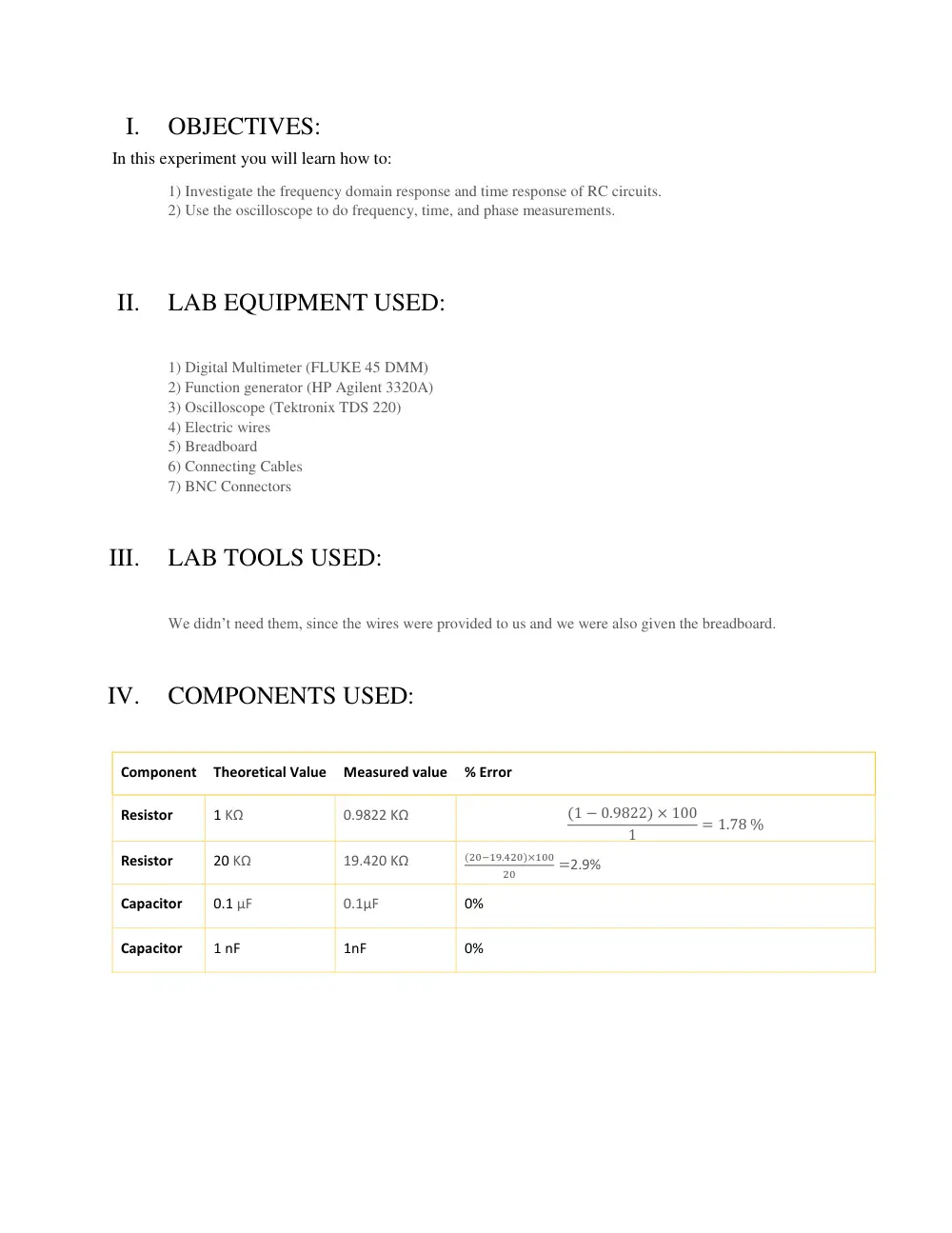COMPONENTS USED: Component Theoretical Value Measured value % Error Resistor 1 KΩ 0.9822 KΩ (1 − 0.9822) × 100 1 = 1.78 % Resistor 20 KΩ 19.420 KΩ (20−19.420)×100 20 =2.9% Capacitor 0.1 µF 0.1µF 0% Capacitor 1 nF 1nF 0% V. EXPERIMENTAL PROCEDURE AND DISCUSSION: A. 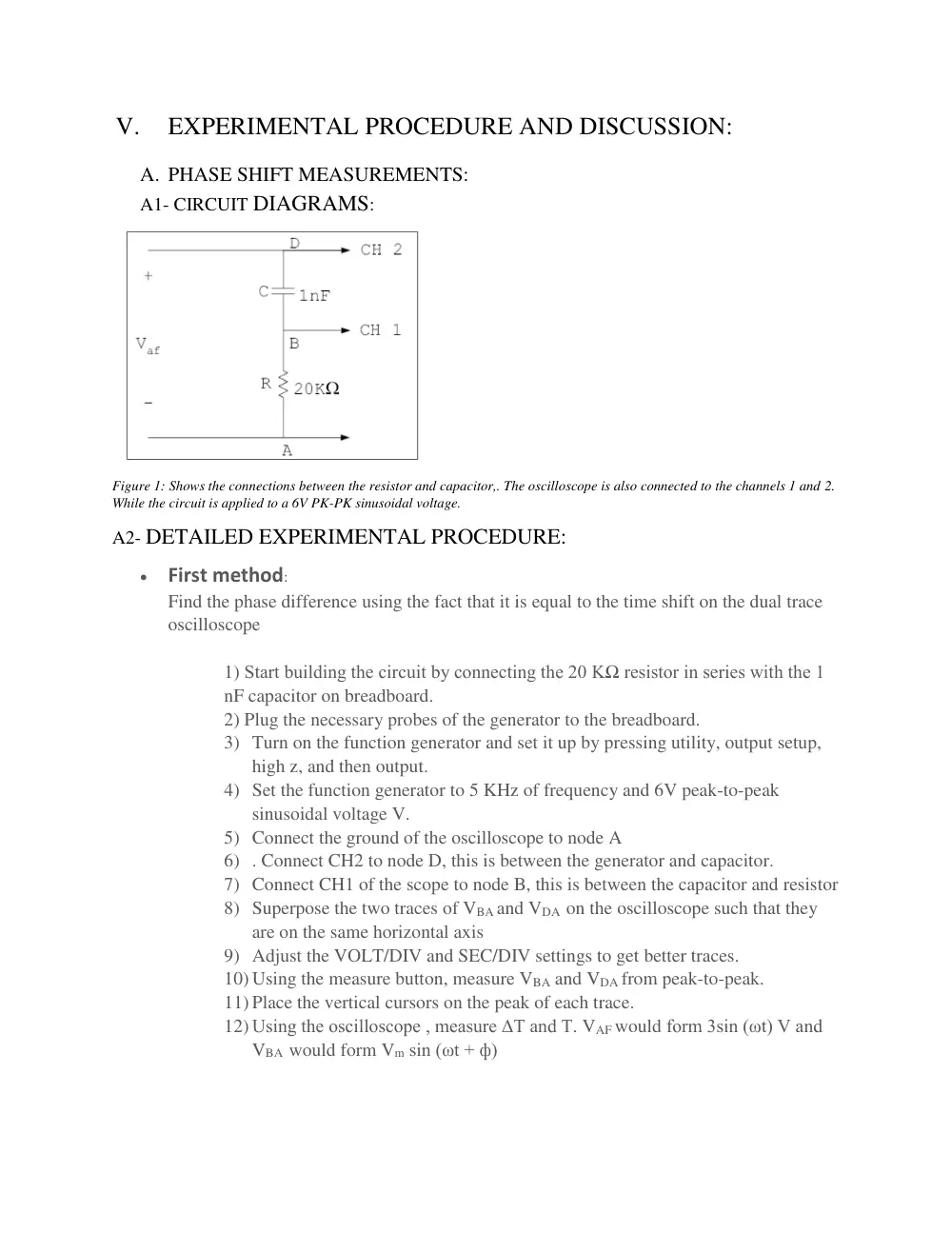PHASE SHIFT MEASUREMENTS: A1- CIRCUIT DIAGRAMS: Figure 1: Shows the connections between the resistor and capacitor,. The oscilloscope is also connected to the channels 1 and 2. While the circuit is applied to a 6V PK-PK sinusoidal voltage. A2- DETAILED EXPERIMENTAL PROCEDURE:  First method: Find the phase difference using the fact that it is equal to the time shift on the dual trace oscilloscope 1) Start building the circuit by connecting the 20 KΩ resistor in series with the 1 nF capacitor on breadboard. 2) Plug the necessary probes of the generator to the breadboard. 3) Turn on the function generator and set it up by pressing utility, output setup, high z, and then output. 4) Set the function generator to 5 KHz of frequency and 6V peak-to-peak sinusoidal voltage V. 5) Connect the ground of the oscilloscope to node A 6) . Connect CH2 to node D, this is between the generator and capacitor. 7) Connect CH1 of the scope to node B, this is between the capacitor and resistor 8) Superpose the two traces of VBA and VDA on the oscilloscope such that they are on the same horizontal axis 9) Adjust the VOLT/DIV and SEC/DIV settings to get better traces. 10) Using the measure button, measure VBA and VDA from peak-to-peak. 11) Place the vertical cursors on the peak of each trace. 12) Using the oscilloscope , measure ΔT and T. VAF would form 3sin (ωt) V and VBA would form Vm sin (ωt + ф)  Second method: Using the Lissajous figure pattern and X-Y mode of function of the oscilloscope: 1) No connections are changed from the previous method 2) Set the sweep rate to X-Y mode. Now VBA and VDA are connected to the X and Y channels of the oscilloscope. 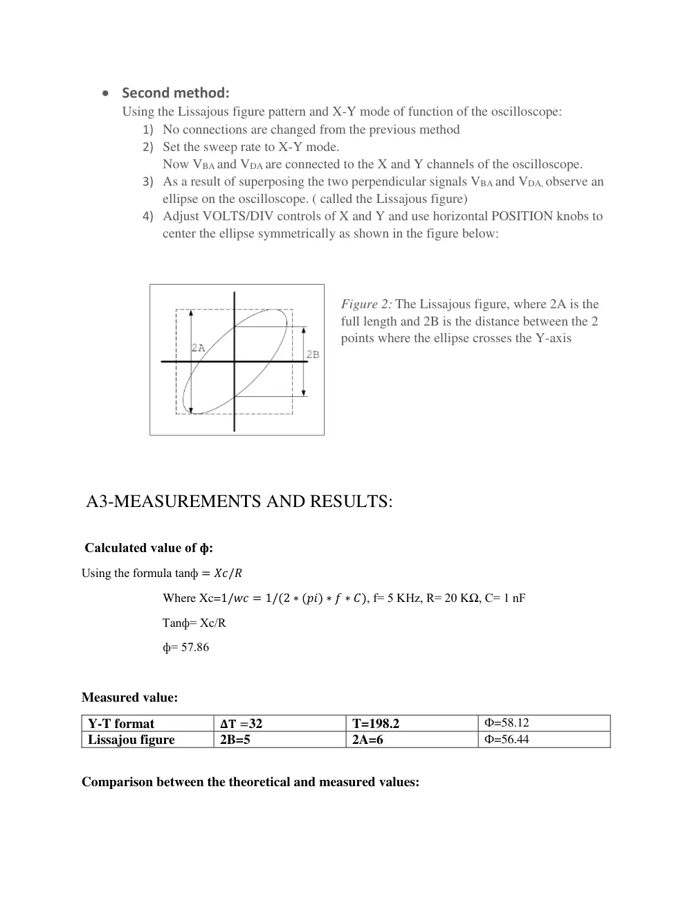3) As a result of superposing the two perpendicular signals VBA and VDA, observe an ellipse on the oscilloscope. ( called the Lissajous figure) 4) Adjust VOLTS/DIV controls of X and Y and use horizontal POSITION knobs to center the ellipse symmetrically as shown in the figure below: Figure 2: The Lissajous figure, where 2A is the full length and 2B is the distance between the 2 points where the ellipse crosses the Y-axis A3-MEASUREMENTS AND RESULTS: Calculated value of ф: Using the formula tanф = 𝑋𝑐/𝑅 Where Xc=1/𝑤𝑐 = 1/(2 ∗ (𝑝𝑖) ∗ 𝑓 ∗ 𝐶), f= 5 KHz, R= 20 KΩ, C= 1 nF Tanф= Xc/R ф= 57.86 Measured value: Y-T format 𝚫𝐓 =32 T=198.2 Ф=58.12 Lissajou figure 2B=5 2A=6 Ф=56.44 Comparison between the theoretical and measured values: The calculated values are close to the measured values. There small difference is due to the reading errors. A4- DISCUSSIONS: Change the frequency of the input and observe how the shape of the ellipse changes. At low frequencies, Zc= infinite, so capacitor acts as open circuit and a vertical line is formed. The ellipse takes the shape of the vertical line. At high frequencies, Zc=0, so the capacitor acts as a short circuit and Vout= RI. This is a linear relationship, so the voltage is represented by a straight line. B. 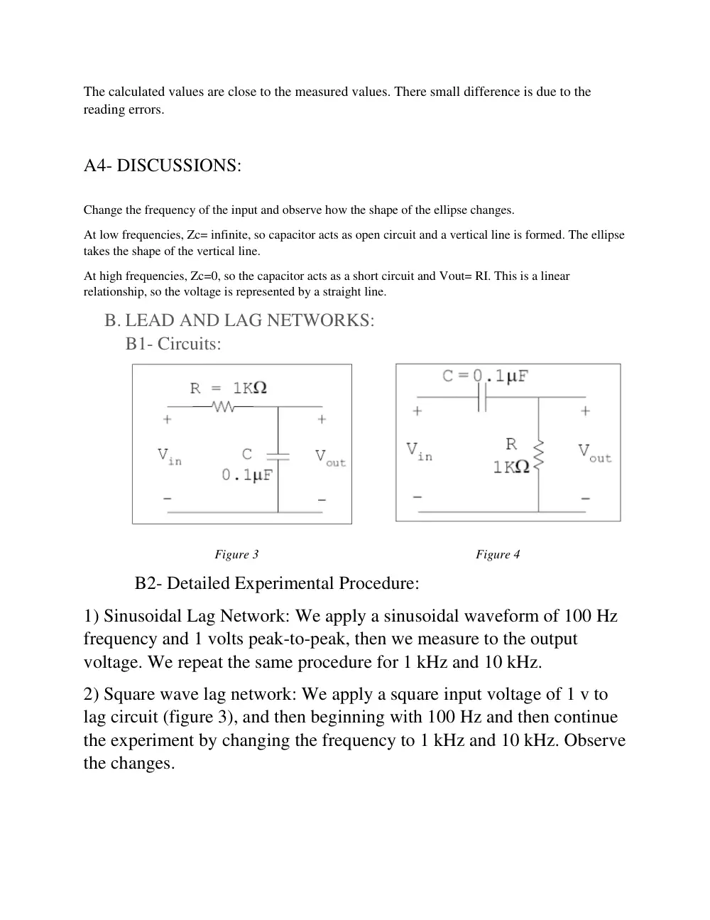LEAD AND LAG NETWORKS: B1- Circuits: Figure 3 Figure 4 B2- Detailed Experimental Procedure: 1) Sinusoidal Lag Network: We apply a sinusoidal waveform of 100 Hz frequency and 1 volts peak-to-peak, then we measure to the output voltage. We repeat the same procedure for 1 kHz and 10 kHz. 2) Square wave lag network: We apply a square input voltage of 1 v to lag circuit (figure 3), and then beginning with 100 Hz and then continue the experiment by changing the frequency to 1 kHz and 10 kHz. Observe the changes. 3) Sinusoidal Lead Network: We apply a sinusoidal waveform of 100 Hz frequency and 1 volts peak-to-peak, then we measure to the output voltage. We repeat the same procedure for 1 kHz and 10 kHz. 4) Square wave lag network: We apply a square input voltage of 1 v to lead circuit (figure 4), and then beginning with 100 Hz and then continue the experiment by changing the frequency to 1 kHz and 10 kHz. Observe the changes. 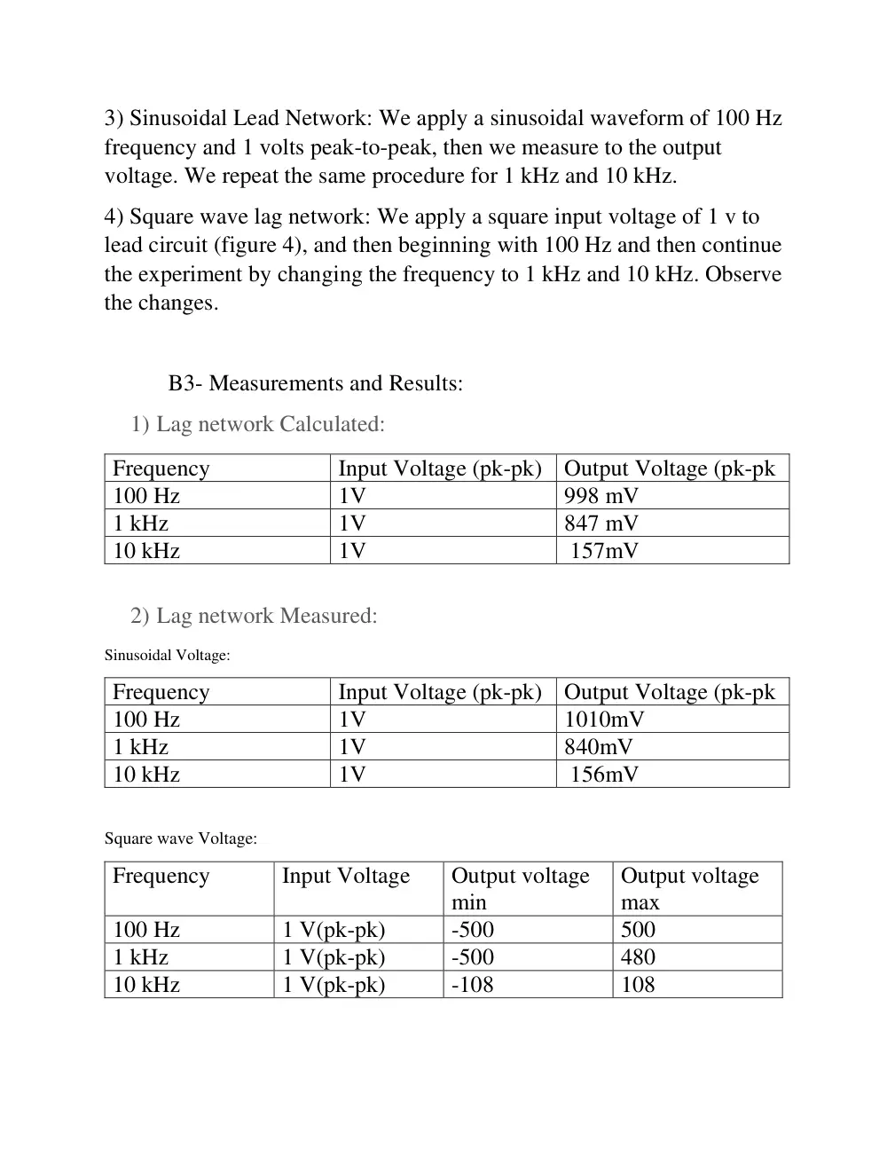B3- Measurements and Results: 1) Lag network Calculated: Frequency Input Voltage (pk-pk) Output Voltage (pk-pk 100 Hz 1V 998 mV 1 kHz 1V 847 mV 10 kHz 1V 157mV 2) Lag network Measured: Sinusoidal Voltage: Frequency Input Voltage (pk-pk) Output Voltage (pk-pk 100 Hz 1V 1010mV 1 kHz 1V 840mV 10 kHz 1V 156mV Square wave Voltage: Frequency Input Voltage Output voltage min Output voltage max 100 Hz 1 V(pk-pk) -500 500 1 kHz 1 V(pk-pk) -500 480 10 kHz 1 V(pk-pk) -108 108 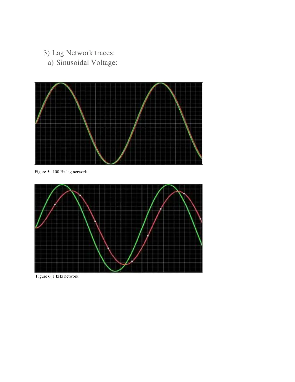3) Lag Network traces: a) Sinusoidal Voltage: Figure 5: 100 Hz lag network Figure 6: 1 kHz network Figure 7: 10 kHz network 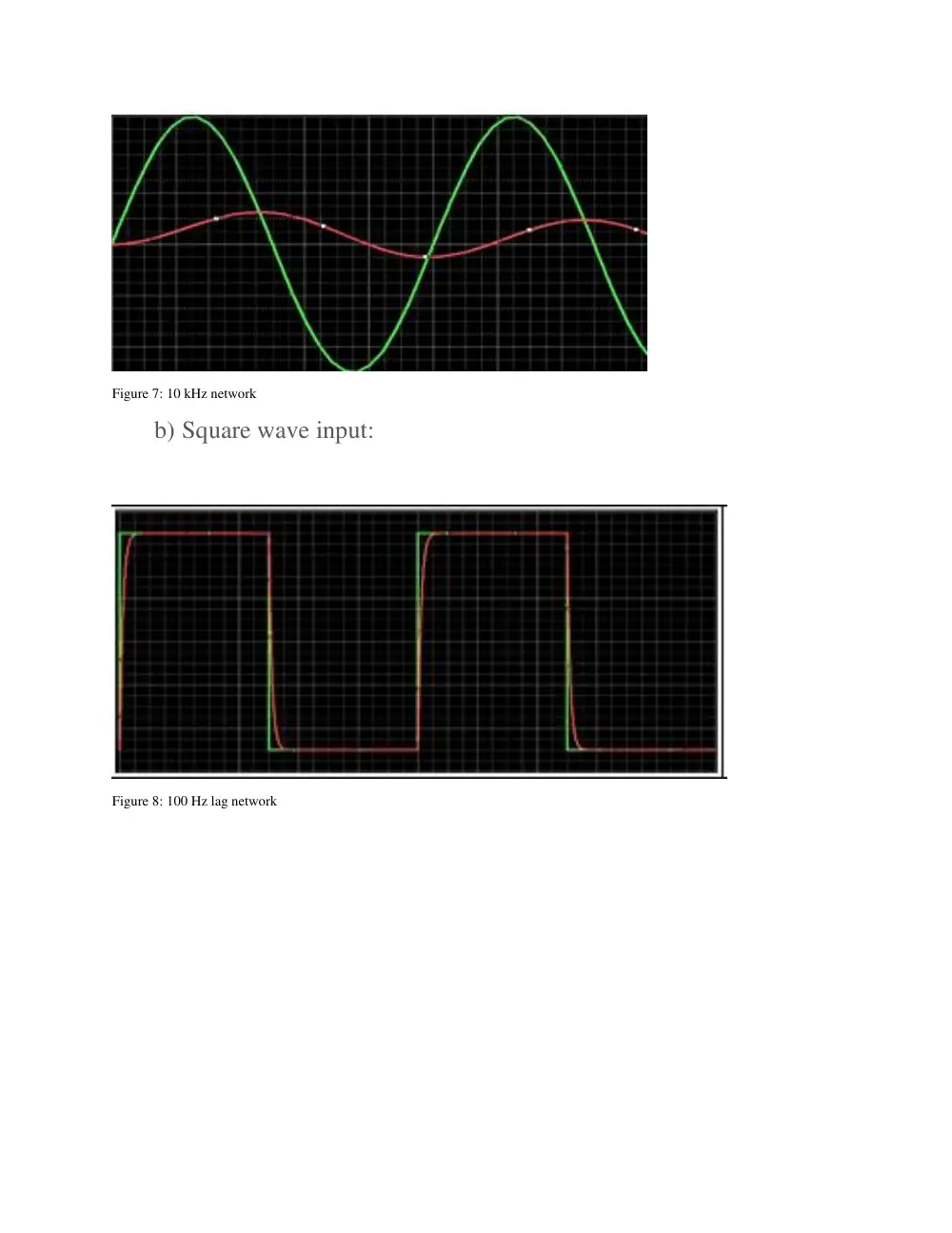b) Square wave input: Figure 8: 100 Hz lag network Figure 9: 1 kHz lag network Figure 10: 10 kHz lag network 4) Lead network calculated: Frequency Input Voltage (pk-pk) Output Voltage (pk-pk 100 Hz 1V 62.7 mV 1 kHz 1V 532 mV 10 kHz 1V 988 mv 5) Lead network Measured: Sinusoidal Voltage: Frequency Input Voltage (pk-pk) Output Voltage (pk-pk 100 Hz 1V 82 mV 1 kHz 1V 580 mV 10 kHz 1V 960 mV Square wave Voltage: Frequency Input Voltage Output voltage min Output voltage max 100 Hz 1 V(pk-pk) -980 960 1 kHz 1 V(pk-pk) -960 960 10 kHz 1 V(pk-pk) -600 580 6) Lead Network traces: a) Sinusoidal Voltage: Figure 11: 100 Hz lead network Figure 12: 1 kHz lead network Figure 13: 10 kHz lead network b) Square wave input: Figure 14: 100 Hz lead network Figure 15: 1 kHz lead network Figure 16: 10 kHz 7) Comparison and errors: The values calculated and the values measured are close. They are not exactly the same because of reading errors on the oscilloscope and perhaps the error of equipment used to perform the procedure. B4- Discussion 1. Lag network, sinusoidal signal 1- In the lag network, the transfer function H(f) is equal to: 1/(1+jwRC). This implies that we are dealing with a low-pass- filter, as when we the frequency goes to infinity, the transfer function is equal to 0, while when the frequency goes to 0, the transfer function is equal to 1. This means this filter lets through small frequencies but blocks big frequencies. When we are dealing with a low-pass-filter or lag network, the cutoff frequency is the highest frequency that manages to pass through filter, this means that any frequency higher than the cutoff frequency is going to be blocked, but any under it will pass. Fco= cutoff frequency Fco= 1/(2πRC) = 1591 hertz 2- When the frequency is low, the output waveforms and the input waveforms are practically identical. However, the more we increase the frequency, the more the output waveforms distorts, and almost equals 0 for very high frequencies. For example, at 100 hz, the waveforms are identical, however when the frequency is equal to 1 Khz, the signal distorts and becomes visibly different than the input signal, yet, they do still resemble each other. As for when the frequency is equal to 10Khz, the output signal is equal to 0 almost, looking nothing like the original signal. 3- The relationship between the RC time constant and the frequency of the sinusoidal input so that the filter does not introduce appreciable attenuation is f < < < 1/RC. This means both f and RC need to be small 4- α= 0 – arctan(2πfRC) This means that when the frequency is small, the phase shift is equal to 0 and when the frequency increase, the phase shift tends to π/2 In conclusion, the previous statements signify that the bigger the frequency is the, the bigger the phase shift will, rising up as high as lagging by π/2 2. Lag network, square signal 1- When the frequency is low, like 100 hertz, the waveforms are almost identical. For frequencies in the range of 1 Khz, the output waveform starts to distort, taking a wave like shape. When the frequencies become relatively high, such as 10 Khz, the output signal becomes triangle shaped. This is due to the fact that when the frequency is small, the period is very high, this means that the frequencies have time to go through the filter before the capacitors charges and becomes an open circuit. The opposite happens when the frequency becomes large, as the period becomes small, giving time for the capacitors to charge before letting in all the frequencies 2- Fourier’s theorem of periodic signals states that all read world signals are sums of sinusoidal components with different frequencies, amplitudes, and phases. Here, we can see that at 100 hertz, the wave is practically identical the first wave, almost a perfect square. However, at 1 khertz, it starts to distort, in a way that it reaches its peak in a sinewave, and then regresses as a cosine wave, in accordance to fourier’s theorem. At 10 khertz, the function assumes triangle waves. As we can see, the higher the frequency, the more distorted the output function is, indicating a low-pass-filter 3- The relationship between the RC time constant and the frequency of the sinusoidal input so that the filter does not introduce appreciable attenuation is f < < < 1/RC. This means both f and RC need to be small. This means the relationship holds for the sinusoidal and square functions 4- In integrators, we only consider high frequencies. That way, the capacitor will not have the time to charge up, implying that the input voltage will be approximately equal to the voltage through the resistor. This means that we can consider a lag network as an integrator. It acts as an integrator at the frequency that corresponds to the RC time constant (f = 1/t) 3. Lead network, sinusoidal signal. 1- In the lead network, the transfer function H(f) is equal to: jwRC/(1+jwRC). This implies that we are dealing with a high- pass-filter, as when we the frequency goes to infinity, the transfer function is equal to 1, while when the frequency goes to 0, the transfer function is equal to 0. This means this filter lets through big frequencies but blocks high frequencies. When we are dealing with a high-pass-filter or lead network, the cutoff frequency is the lowest frequency that manages to pass through filter, this means that any frequency lower than the cutoff frequency is going to be blocked, but any over it will pass. Fco= cutoff frequency Fco= 1/(2πRC) =1591 hertz 2- When the frequency is high, the output waveforms and the input waveforms are practically identical. However, the more we decrease the frequency, the more the output waveforms distorts, and almost equals 0 for very low frequencies. For example, at 10 khz, the waveforms are identical, however when the frequency is equal to 1 Khz, the signal distorts and becomes visibly different than the input signal, yet, they do still resemble each other. As for when the frequency is equal to 100 hz, the output signal is equal to 0 almost, looking nothing like the original signal. 3- The relationship between the RC time constant and the frequency of the sinusoidal input so that the filter does not introduce appreciable attenuation is f > > >1/RC. This means both f and RC need to be large 4- α= 90 – arctan(2πfRC) This means that when the frequency is small, the phase shift is equal to π/2 and when the frequency increase, the phase shift tends to 0 In conclusion, the previous statements signify that the bigger the frequency is, the smaller the phase shift will. However, the smaller the frequency is, the bigger the phase shift will be, reaching up to a difference of π/2 4. Lead network, square signal. 1- In the lead network, the transfer function H(f) is equal to: jwRC/(1+jwRC). This implies that we are dealing with a high- pass-filter, as when we the frequency goes to infinity, the transfer function is equal to 1, while when the frequency goes to 0, the transfer function is equal to 0. This means this filter lets through big frequencies but blocks high frequencies. This is due to the fact that when the frequency is so high, the period is very low. This means that the capacitor doesn’t have enough time to charge, and no voltage is remarked on it. However, the lower the frequency, the higher the period, giving the capacitor time to charge, creating a voltage, causing the distortions 2- Fourier’s theorem of periodic signals states that all read world signals are sums of sinusoidal components with different frequencies, amplitudes, and phases. Here, we can see that at 10 khertz, the wave is practically identical to the first wave, almost a perfect square. However, at 1 khertz, it starts to distort, in a way that it reaches its peak in a sinewave, and then regresses as a cosine wave, in accordance to fourier’s theorem. At 100 hertz, the function assumes triangle waves. As we can see, the lower the frequency, the more distorted the output function is, indicating a high-pass-filter 3- The relationship between the RC time constant and the frequency of the sinusoidal input so that the filter does not introduce appreciable attenuation is f > > >1/RC. This means both f and RC need to be large. Thus, the relationship is true for the sinusoidal and square functions. 4- Differentiators blocks low frequencies and lets through large frequencies. This is due to the fact that the high frequencies decrease the reactance of capacitors. This implies that at high frequencies, the capacitor acts as a short circuit, and the inputs and outputs become identical. It acts as an integrator at the frequency that corresponds to the RC time constant (f = 1/t) . VI. Mistakes and Problems we have faced: We faced the problem of reading the values on the oscilloscope because they were constantly changing. It was hard to read the divisions on the oscilloscope accurately. VII. Signature I have neither given nor received aid on this report nor have I concealed any violation of the AUB student code of conduct