EECE 310L Lab 8, Fall 2011

EECE 310L : Electric Circuits Laboratory Experiment 8 1 A m e r i c a n   U n i v e r s i t y   o f   B e i r u t Fall 2011 Experiment 8 Op‐Amp Circuits EECE 310L : Electric Circuits Laboratory Experiment 8 2 Table of Contents I. Objectives ................................................................................................................................ 3 II. Material and Procedure ...................................................................................................... 3 A. Inverting Amplifier .......................................................................................................... 3 A1. Inverting amplifier procedure 1: Theoretical Vs measured .................................. 3 A2. Inverting amplifier procedure 2: BAndwidth ............................................................... 4 A3. Inverting amplifier procedure 3: High Input ................................................................ 4 B. Non­Inverting Amplifier ................................................................................................ 5 B1. non‐Inverting amplifier procedure 1: Theoretical Vs measured ........................ 5 B2. non‐Inverting amplifier procedure 2: BAndwidth ..................................................... 6 C. Unity­Gain Non­Inverting Amplifier........................................................................... 6 C1. Unity amplifier procedure ..................................................................................................... 6 D. Inverting Adder ................................................................................................................ 7 E. Integrator ........................................................................................................................... 8 E1. Integrator: theoretical calculation ..................................................................................... 8 E2. Integrator: Theoretical vs measured ................................................................................ 8 E3. Integrator: Bandwidth ............................................................................................................. 9 F. Differentiator .................................................................................................................... 9 F1. differentiator: theoretical calculation ........................................................................... 10 F2. Integrator: Theoretical vs measured ............................................................................. 10 III.  Outcomes .............................................................................................................................. 10 EECE 310L : Electric Circuits Laboratory Experiment 8 3 I. OBJECTIVES In  this  experiment  you  will  investigate  the  characteristics  of  the  following  op‐amp circuits: • inverting amplifier • non‐inverting amplifier • unit‐gain buffer • inverting adder • integrator • differentiator II. MATERIAL AND PROCEDURE A. 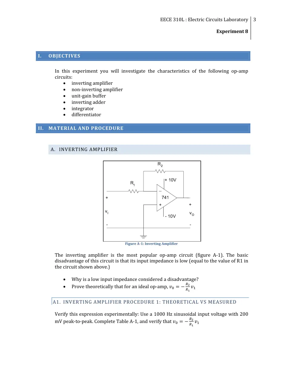INVERTING AMPLIFIER Figure  A­1: Inverting Amplifier The  inverting  amplifier  is  the  most  popular  op‐amp  circuit  (figure  A‐1).  The  basic disadvantage of this circuit is that its input impedance is low (equal to the value of R1 in the circuit shown above.) • Why is a low input impedance considered a disadvantage? • Prove theoretically that for an ideal op‐amp, �� � � �� �� �� A1. INVERTING AMPLIFIER PROCEDURE 1: THEORETICAL VS MEASURED Verify this expression experimentally: Use a 1000 Hz sinusoidal input voltage with 200 mV peak‐to‐peak. 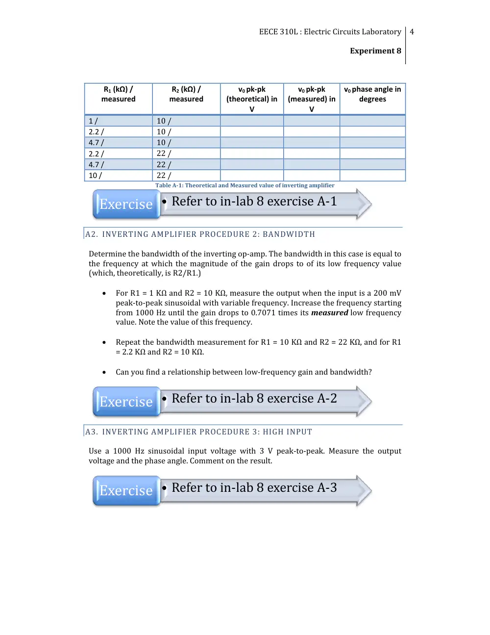Complete Table A‐1, and verify that �� � � �� �� �� EECE 310L : Electric Circuits Laboratory Experiment 8 4 R1 (kΩ) / measured R2 (kΩ) / measured v0 pk‐pk (theoretical) in V v0 pk‐pk (measured) in V v0 phase angle in degrees 1 / 10 / 2.2 / 10 / 4.7 / 10 / 2.2 / 22 / 4.7 / 22 / 10 / 22 / Table  A­1: Theoretical and Measured value of inverting amplifier A2. INVERTING AMPLIFIER PROCEDURE 2: BANDWIDTH Determine the bandwidth of the inverting op‐amp. The bandwidth in this case is equal to the frequency at which the magnitude of the gain drops to of its low frequency value (which, theoretically, is R2/R1.) • For R1 = 1 KΩ and R2 = 10 KΩ, measure the output when the input is a 200 mV peak‐to‐peak sinusoidal with variable frequency. Increase the frequency starting from 1000 Hz until the gain drops to 0.7071 times its measured low frequency value. Note the value of this frequency. • Repeat the bandwidth measurement for R1 = 10 KΩ and R2 = 22 KΩ, and for R1 = 2.2 KΩ and R2 = 10 KΩ. • Can you find a relationship between low‐frequency gain and bandwidth? A3. INVERTING AMPLIFIER PROCEDURE 3: HIGH INPUT Use  a  1000  Hz  sinusoidal  input  voltage  with  3  V  peak‐to‐peak.  Measure  the  output voltage and the phase angle. Comment on the result. 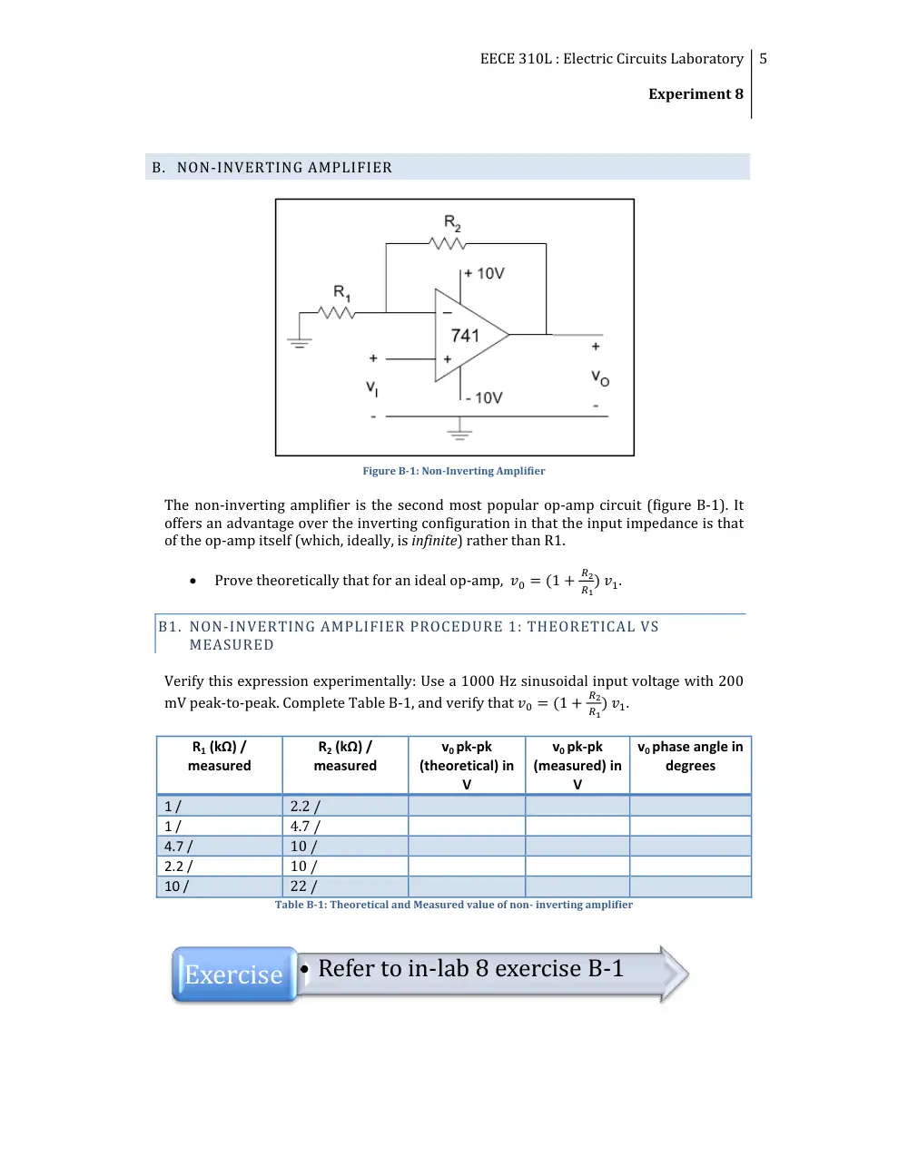• Refer to in‐lab 8 exercise A‐1 Exercise • Refer to in‐lab 8 exercise A‐2 Exercise Exercise • Refer to in‐lab 8 exercise A‐3 EECE 310L : Electric Circuits Laboratory Experiment 8 5 B. NON‐INVERTING AMPLIFIER Figure  B­1: Non­Inverting Amplifier The non‐inverting amplifier is the second most popular op‐amp circuit (figure B‐1). It offers an advantage over the inverting configuration in that the input impedance is that of the op‐amp itself (which, ideally, is infinite) rather than R1. • Prove theoretically that for an ideal op‐amp,  �� � �1 � �� ��� ��. B1. NON‐INVERTING AMPLIFIER PROCEDURE 1: THEORETICAL VS MEASURED Verify this expression experimentally: Use a 1000 Hz sinusoidal input voltage with 200 mV peak‐to‐peak. Complete Table B‐1, and verify that �� � �1 � �� ��� ��. R1 (kΩ) / measured R2 (kΩ) / measured v0 pk‐pk (theoretical) in V v0 pk‐pk (measured) in V v0 phase angle in degrees 1 / 2.2 / 1 / 4.7 / 4.7 / 10 / 2.2 / 10 / 10 / 22 / Table  B­1: Theoretical and Measured value of non­ inverting amplifier Exercise • Refer to in‐lab 8 exercise B‐1 EECE 310L : Electric Circuits Laboratory Experiment 8 6 B2. NON‐INVERTING AMPLIFIER PROCEDURE 2: BANDWIDTH Determine  the  bandwidth  of  the  non‐inverting  op‐amp.  As  before,  the  bandwidth  is equal  to  the  frequency  at  which  the  magnitude  of  the  gain �� �� drops  to � √� of  its  low frequency value (which, theoretically, is 1 � �� ��) • For R1 = 1 KΩ and R2 = 4.7 KΩ, measure the output when the input is a 200 mV peak‐to‐peak sinusoidal with variable frequency. Increase the frequency starting from 1000 Hz until the gain drops to 0.7071 times its measured low frequency value. Note the value of this frequency. • Repeat the bandwidth measurement for R1 = 10 KΩ and R2 = 22 KΩ. 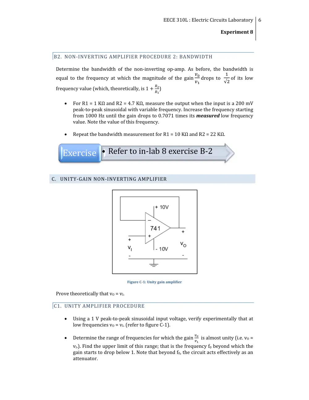C. UNITY‐GAIN NON‐INVERTING AMPLIFIER Figure  C­1: Unity gain amplifier Prove theoretically that vO = vI. C1. UNITY AMPLIFIER PROCEDURE • Using a 1 V peak‐to‐peak sinusoidal input voltage, verify experimentally that at low frequencies vO = vI. (refer to figure C‐1). • Determine the range of frequencies for which the gain �� ��  is almost unity (i.e. vO = vI.). Find the upper limit of this range; that is the frequency f0 beyond which the gain starts to drop below 1. Note that beyond f0, the circuit acts effectively as an attenuator. Exercise • Refer to in‐lab 8 exercise B‐2 EECE 310L : Electric Circuits Laboratory Experiment 8 7 • Determine the bandwidth of the unity‐gain non‐inverting op‐amp. As before, the bandwidth is equal to the frequency at which the magnitude of the gain �� �� drops to � √�   (since the low‐frequency gain is theoretically equal to 1.) • How does this bandwidth compare with that of the non‐inverting amplifier? 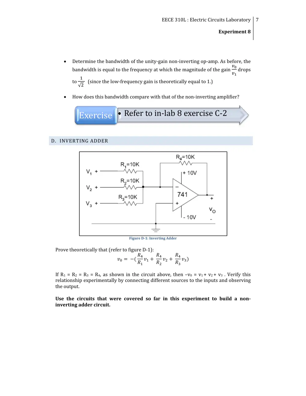D. INVERTING ADDER Figure  D­1: Inverting Adder Prove theoretically that (refer to figure D‐1): �� � �� �� �� �� � �� �� �� � �� �� ��� If R1 = R2 = R3 = R4, as shown in the circuit above, then –v0 = v1 + v2 + v3 . Verify this relationship experimentally by connecting different sources to the inputs and observing the output. Use  the  circuits  that  were  covered  so  far  in  this  experiment  to  build  a  non­ inverting adder circuit. 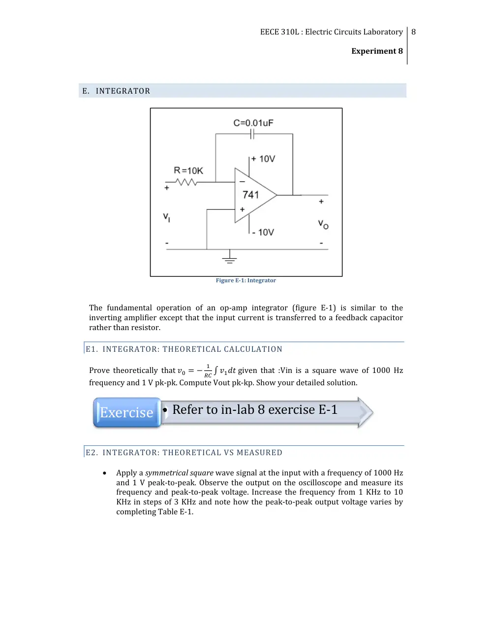Exercise • Refer to in‐lab 8 exercise C‐2 EECE 310L : Electric Circuits Laboratory Experiment 8 8 E. INTEGRATOR Figure  E­1: Integrator The  fundamental  operation  of  an  op‐amp  integrator  (figure  E‐1)  is  similar  to  the inverting amplifier except that the input current is transferred to a feedback capacitor rather than resistor. E1. INTEGRATOR: THEORETICAL CALCULATION Prove  theoretically  that �� � � � �� � ���� given  that  :Vin  is  a  square  wave  of  1000  Hz frequency and 1 V pk‐pk. Compute Vout pk‐kp. Show your detailed solution. E2. INTEGRATOR: THEORETICAL VS MEASURED • Apply a symmetrical square wave signal at the input with a frequency of 1000 Hz and 1 V peak‐to‐peak. Observe the output on the oscilloscope and measure its frequency and peak‐to‐peak voltage. Increase the frequency from 1 KHz to 10 KHz in steps of 3 KHz and note how the peak‐to‐peak output voltage varies by completing Table E‐1. 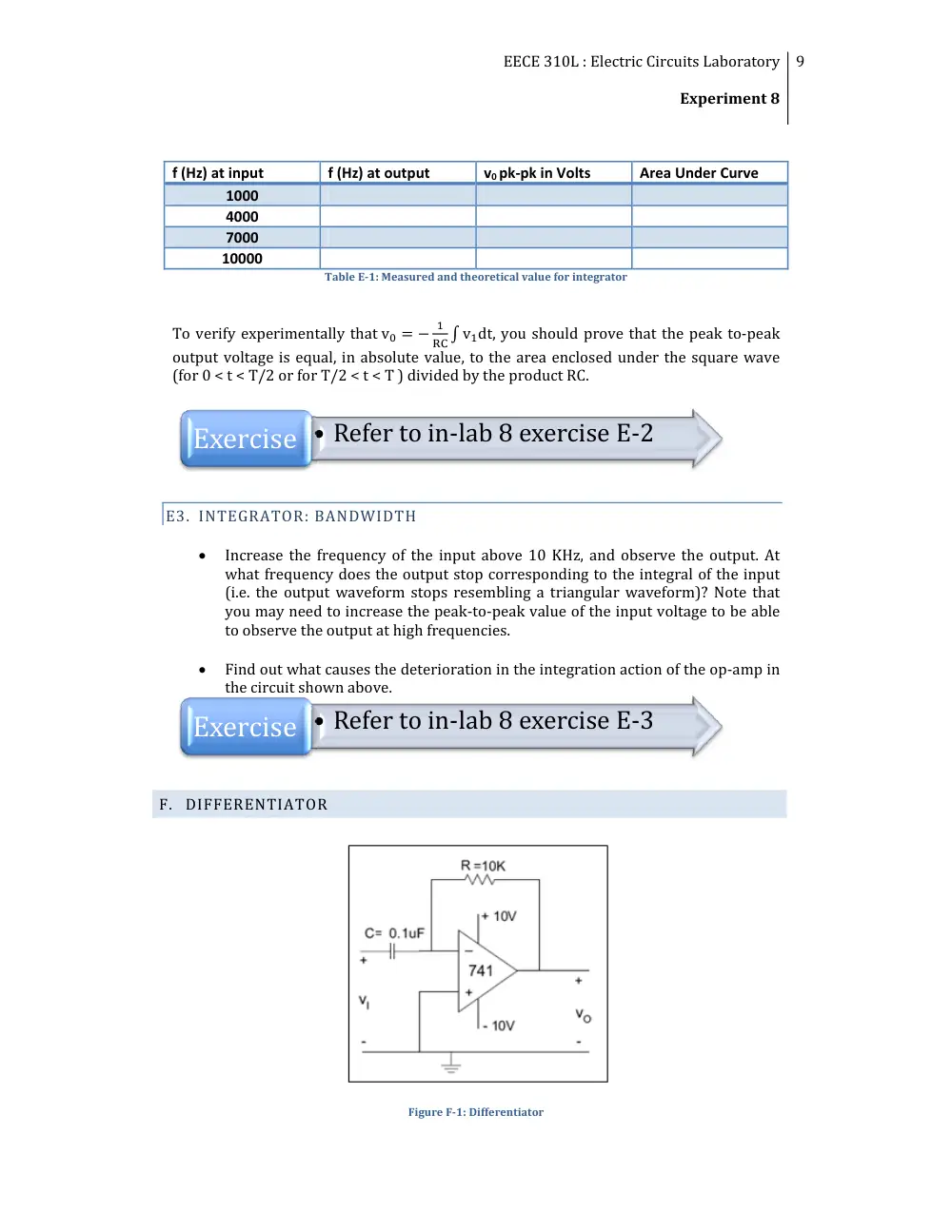Exercise • Refer to in‐lab 8 exercise E‐1 EECE 310L : Electric Circuits Laboratory Experiment 8 9 f (Hz) at input f (Hz) at output v0 pk‐pk in Volts Area Under Curve 1000 4000 7000 10000 Table  E­1: Measured and theoretical value for integrator To verify experimentally that v� � � � RC � v�dt, you should prove that the peak to‐peak output voltage is equal, in absolute value, to the area enclosed under the square wave (for 0 < t < T/2 or for T/2 < t < T ) divided by the product RC. E3. INTEGRATOR: BANDWIDTH • Increase the frequency of the input above 10 KHz, and observe the output. At what frequency does the output stop corresponding to the integral of the input (i.e. the output waveform stops resembling a triangular waveform)? Note that you may need to increase the peak‐to‐peak value of the input voltage to be able to observe the output at high frequencies. • Find out what causes the deterioration in the integration action of the op‐amp in the circuit shown above. F. 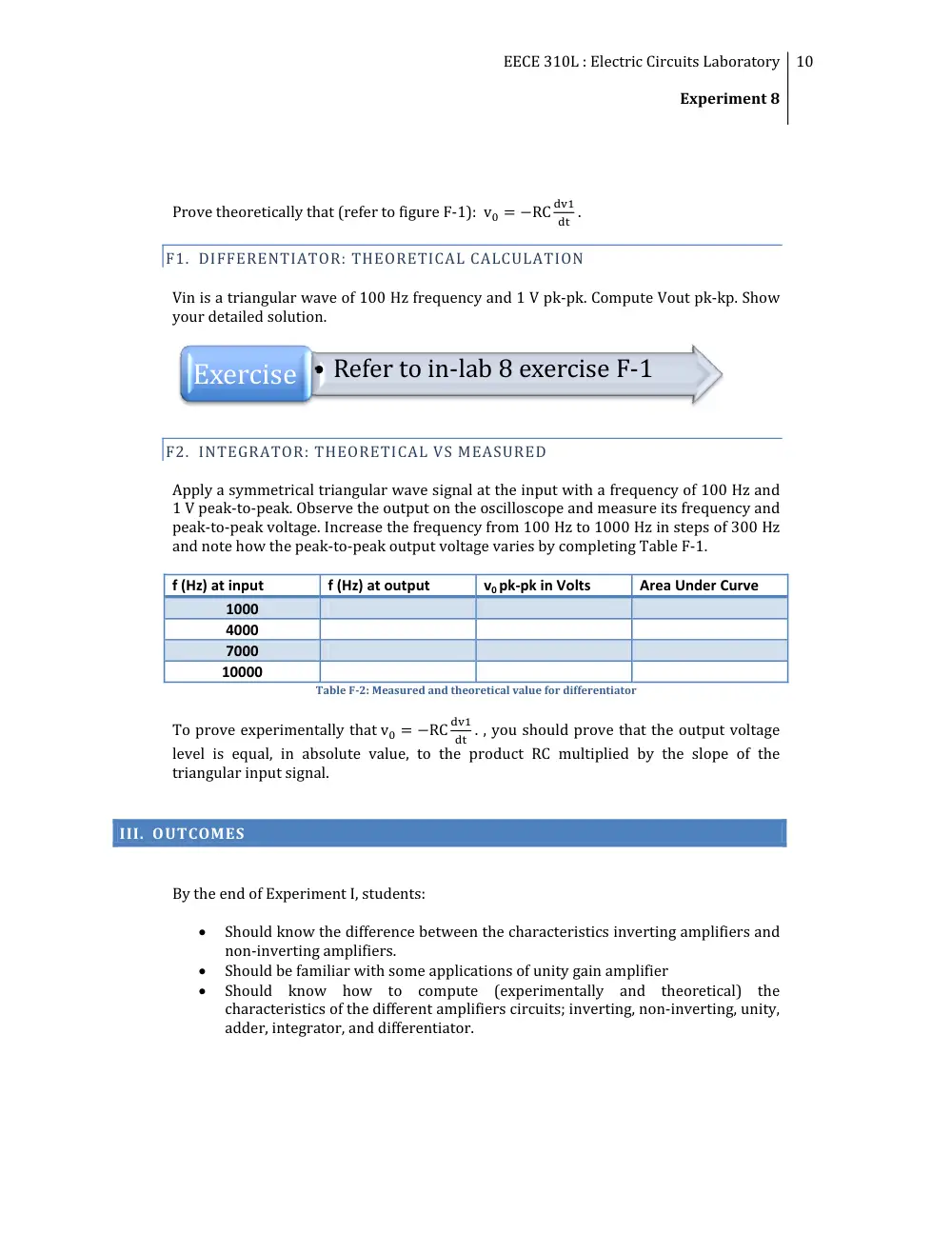DIFFERENTIATOR Figure  F­1: Differentiator • Refer to in‐lab 8 exercise E‐2 Exercise Exercise • Refer to in‐lab 8 exercise E‐3 EECE 310L : Electric Circuits Laboratory Experiment 8 10 Prove theoretically that (refer to figure F‐1):  v� � �RC ��� ��  . F1. DIFFERENTIATOR: THEORETICAL CALCULATION Vin is a triangular wave of 100 Hz frequency and 1 V pk‐pk. Compute Vout pk‐kp. Show your detailed solution. F2. INTEGRATOR: THEORETICAL VS MEASURED Apply a symmetrical triangular wave signal at the input with a frequency of 100 Hz and 1 V peak‐to‐peak. Observe the output on the oscilloscope and measure its frequency and peak‐to‐peak voltage. Increase the frequency from 100 Hz to 1000 Hz in steps of 300 Hz and note how the peak‐to‐peak output voltage varies by completing Table F‐1. f (Hz) at input f (Hz) at output v0 pk‐pk in Volts Area Under Curve 1000 4000 7000 10000 Table  F­2: Measured and theoretical value for differentiator To prove experimentally that v� � �RC ��� ��  . , you should prove that the output voltage level  is  equal,  in  absolute  value,  to  the  product  RC  multiplied  by  the  slope  of  the triangular input signal. III. OUTCOMES By the end of Experiment I, students: • Should know the difference between the characteristics inverting amplifiers and non‐inverting amplifiers. • Should be familiar with some applications of unity gain amplifier • Should  know  how  to  compute  (experimentally  and  theoretical)  the characteristics of the different amplifiers circuits; inverting, non‐inverting, unity, adder, integrator, and differentiator. Exercise • Refer to in‐lab 8 exercise F‐1