EECE 330 Lecture 9, Fall 2010

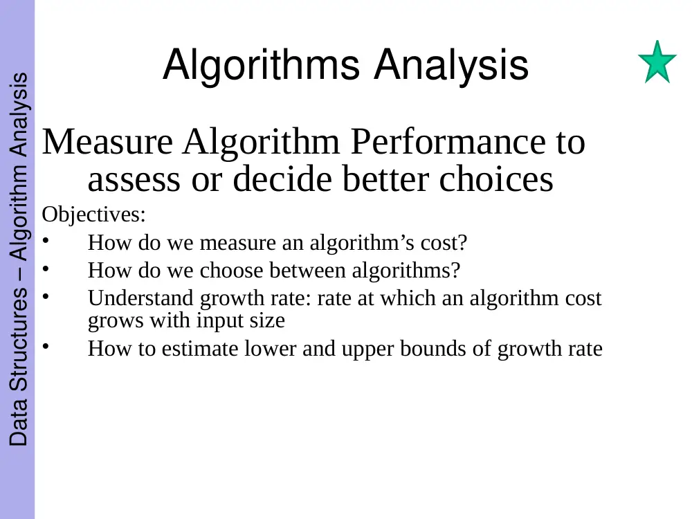
Data Structures – Algorithm Analysis Algorithm Analysis Ch. 3, (and some from :2, 14) Data Structures – Algorithm Analysis Algorithms Analysis Measure Algorithm Performance to assess or decide better choices Objectives: • How do we measure an algorithm’s cost? • How do we choose between algorithms? • Understand growth rate: rate at which an algorithm cost grows with input size • How to estimate lower and upper bounds of growth rate Data Structures – Algorithm Analysis How to Measure Efficiency? • Empirical comparison: Implement and run programs • Asymptotic Algorithm Analysis : Algorithm Analysis Critical resources: Time and Space For most algorithms, running time depends on “size” of the input. Running time is expressed as T(n) for some function T on input size n. 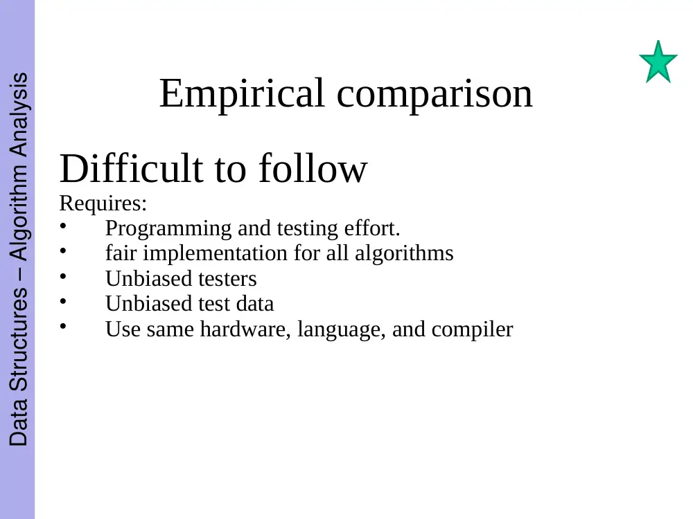Data Structures – Algorithm Analysis Empirical comparison Difficult to follow Requires: • Programming and testing effort. 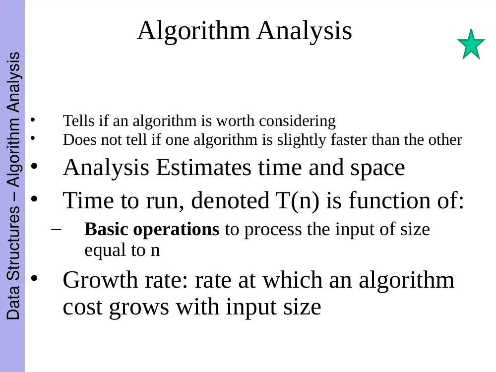• fair implementation for all algorithms • Unbiased testers • Unbiased test data • Use same hardware, language, and compiler Data Structures – Algorithm Analysis Algorithm Analysis • Tells if an algorithm is worth considering • Does not tell if one algorithm is slightly faster than the other • Analysis Estimates time and space • Time to run, denoted T(n) is function of: – Basic operations to process the input of size equal to n • Growth rate: rate at which an algorithm cost grows with input size Data Structures – Algorithm Analysis Examples of Growth Rate Example 1. // Find largest value int largest(int array[], int n) { int currlarge = 0; // Largest value seen for (int i=1; i<n; i++) if (array[currlarge] < array[i]) currlarge = i; return currlarge; } Concern is comparison: T(n)= ? 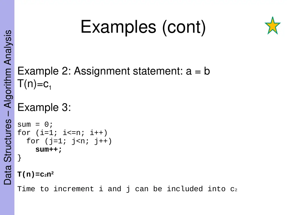T(n)= cn Data Structures – Algorithm Analysis Examples (cont) Example 2: Assignment statement: a = b T(n)=c1 Example 3: sum = 0; for (i=1; i<=n; i++) for (j=1; j<n; j++) sum++; } T(n)=c2n2 Time to increment i and j can be included into c2 Data Structures – Algorithm Analysis Growth Rate Graph Poor Performance in order: 1.Linear 2.nlogn 3.Quadratic 4.Exponential Data Structures – Algorithm Analysis Growth Rate (cont) Using linear search with n=1G: time=c1230 Using instead Binary search (without accounting for Sorting): time= c’ x 30 , significant improvement Faster Alg. 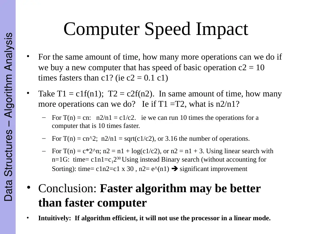Data Structures – Algorithm Analysis Computer Speed Impact • For the same amount of time, how many more operations can we do if we buy a new computer that has speed of basic operation c2 = 10 times fasters than c1? (ie c2 = 0.1 c1) • Take T1 = c1f(n1); T2 = c2f(n2). In same amount of time, how many more operations can we do? Ie if T1 =T2, what is n2/n1? – For T(n) = cn: n2/n1 = c1/c2. ie we can run 10 times the operations for a computer that is 10 times faster. – For T(n) = cn^2; n2/n1 = sqrt(c1/c2), or 3.16 the number of operations. – For T(n) = c*2^n; n2 = n1 + log(c1/c2), or n2 = n1 + 3. Using linear search with n=1G: time= c1n1=c1230 Using instead Binary search (without accounting for Sorting): time= c1n2=c1 x 30 , n2= e^(n1)  significant improvement • Conclusion: Faster algorithm may be better than faster computer • Intuitively: If algorithm efficient, it will not use the processor in a linear mode. Data Structures – Algorithm Analysis Best, Worst, Average Cases Not all inputs of a given size take the same time to run. Which Case to Use for Alg Analysis? • Best case: rarely occurs, too optimistic. Sometimes used if it occurs frequently • Worst case: Important for real time applications • Average time: Appears to be the fairest measure, but difficult to determine: input data distribution NOTE: These cases refer to same data size, different data sets. Data Structures – Algorithm Analysis Asymptotic Analysis • No major effect with faster computer or compiler • Constant factors cause only a shift of the growth rate curves and their crossing points • Asymptotic analysis: for large n, ignore constants, simplifies analysis. Data Structures – Algorithm Analysis Performance Bounds Algorithm Performance O(_): Upper Bound (_): Lower Bound Data Structures – Algorithm Analysis Upper Bounds: Big-Oh We state: “This algorithm has an upper bound of f(n) to its growth rate” Or simply state: “This algorithm is in O(f(n))” Definition: For T(n) a non-negatively valued function, T(n) is in O(f(n)) if there exist two positive constants c and n0 such that T(n)  cf(n) for all n > n0. Usage: The algorithm is in O(n2) in a particular case [best, or average, or worst] Choose tightest bound Data Structures – Algorithm Analysis Big-Oh Notation (continued) Example 1: T(n) = c1n2 + c2n in the average case (c1 and c2  0). Since c1n2 + c2n  c1n2 + c2n2  T(n)  cn2 where c=c1+c2  T(n) is in O(n2). Example 2: Finding value X in an array. T(n) = csn/2 in the average case. For all values of n > 1, csn/2  csn.  T(n) is in O(n). Example 3: T(n) = c.  T(n) is in O(1). Data Structures – Algorithm Analysis Lower Bound: Big-Omega Definition: For T(n) a non-negatively valued function, T(n) is in (g(n)) if there exist two positive constants c and n0 such that T(n)  cg(n) for all n > n0. Meaning: For all data sets big enough (i.e., n > n0), the algorithm always executes in more than cg(n) steps. Data Structures – Algorithm Analysis Big-Omega Example T(n) = c1n2 + c2n. c1n2 + c2n  c1n2 for all n > 1. T(n) >= cn2 for c = c1 and n0 = 1. Therefore, T(n) is in (n2) by definition. Data Structures – Algorithm Analysis Theta Notation • When big-Oh and  meet, we indicate this by using  (big-Theta) notation. In this case we have a perfect analysis of the algorithm: Cases in this course • Definition: An algorithm is said to be (h(n)) if it is in O(h(n)) and it is in (h(n)). • Some algorithms have no  analysis Data Structures – Algorithm Analysis Simplifying Rules 1. If T(n) is in O(g(n)) and g(n) is in O(h(n)), then T(n) is in O(h(n)). 2. Ignore constants. If T(n) is in O(kg(n)) for any constant k > 0, then T(n) is in O(g(n)). 3. Drop low order terms. If T1(n) is in O(g1(n)) and T2(n) is in O(g2(n)), then (T1+T2)(n) is in O(max(g1(n), g2(n))). 4. Useful for analyzing loops. If T1(n) is in O(g1(n)) and T2(n) is in O(g2(n)) then T1(n) T2(n) is in O(g1(n)g2(n)). Data Structures – Algorithm Analysis Assignment Example 1: a = b; Example 2: sum = 0; for (i=1; i<=n; i++) sum += n; Example 3: sum = 0; for (j=1; j<=n; j++) for (i=1; i<=j; i++) sum++; for (k=0; k<n; k++) A[k] = k; Example 4: sum1 = 0; for (i=1; i<=n; i++) for (j=1; j<=n; j++) sum1++; sum2 = 0; for (i=1; i<=n; i++) for (j=1; j<=i; j++) sum2++; Example 5: sum1 = 0; for (k=1; k<=n; k*=2) //log n times for (j=1; j<=n; j++) // n times sum1++; // (nlogn) Determine O, , and  for all examples below as they apply. Data Structures – Algorithm Analysis Other Control Statements while loop: Analyze like a for loop. if statement: Take greater complexity of then/else clauses. switch statement: Take complexity of most expensive case. Function/Method call: Complexity of the Function/Method. Data Structures – Algorithm Analysis Analyzing Problems A problem may be solved by multiple algorithms Upper bound of the problem: Upper bound of best known algorithm. ie: To say that the problem can not perform worse than a certain bound. The worse case performance for the problem can not be worse than the best algorithm, since we know that one solves it. Lower bound of the problem : Lower bound for every possible algorithm. ie: To say that a problem must perform better than a lower bound means every algorithm has to do that. Data Structures – Algorithm Analysis Analyzing Problems: Example Example: Sorting requires at least cn time since each element is examined once. 1. Bubble sort: O(n2). 2. A better sort (Quicksort, Mergesort, Heapsort, etc.): O(n log n). 3. We prove later that sorting is (n log n). Conclusion: ?? Sorting is (n log n). Data Structures – Algorithm Analysis Space Bounds Space bounds can also be analyzed with asymptotic complexity analysis.  Time is affected mostly by algorithm design  Space is affected mostly by the data structures used Data Structures – Algorithm Analysis Space/Time Tradeoff Principle One can often reduce time if one is willing to sacrifice space, or vice versa. • Encoding or packing information (less space but slower execution) - Example: zipped files • Table lookup (more space but faster execution) - Example Factorials Disk-based Space/Time Tradeoff Principle: (opposite to above) The smaller you make the disk storage requirements, the faster your program will run. Data Structures – Algorithm Analysis Mathematical Background – Ch. 2 Data Structures – Algorithm Analysis Mathematical Background Recursion Summation and Recurrence Relations (example p. 68, and recurrence relation, examples 2.7 and 2.12) (example p. 68-69 – binary search Induction Proofs Data Structures – Algorithm Analysis C++ Programming: Program Design Including Data Structures, Third Edition 28 Recursive Definitions • Recursion: solving a problem by reducing it to smaller versions of itself • 0! = 1 (1) n! = n x (n-1)! if n > 0 (2) • The definition of factorial in equations (1) and (2) is called a recursive definition • Equation (1) is called the base case • Equation (2) is called the general case Data Structures – Algorithm Analysis C++ Programming: Program Design Including Data Structures, Third Edition 29 • Example: factorial n! = n * ( n – 1 ) * ( n – 2 ) * … * 1 – Recursive relationship ( n! = n * ( n – 1 )! ) 5! = 5 * 4! 4! = 4 * 3! 3! = 3 * 2! 2! = 2 * 1! 1! = 1 – Base case (1! = 0! = 1) 1 2 6 24 120 Data Structures – Algorithm Analysis C++ Programming: Program Design Including Data Structures, Third Edition 30 Recursive Definitions (continued) • Recursive definition: defining a problem in terms of a smaller version of itself – Every recursive definition must have one (or more) base cases – The general case must eventually reduce to a base case – The base case stops the recursion Data Structures – Algorithm Analysis C++ Programming: Program Design Including Data Structures, Third Edition 31 Recursive Function Example int fact (int num) { if (num == 0) return 1; else return num*fact(num-1); } Data Structures – Algorithm Analysis Mathematical Background Recursion Summation and Recurrence Relations (example p. 68, and recurrence relation, examples 2.7 and 2.12) (example p. 68-69 – binary search Induction Proofs Data Structures – Algorithm Analysis Recurrence and Summation Example • Analysis of fact(): T(n) = T(n-1) + 1 • This relation is called a recurrence • Ideally, we want a closed form for it.. • Expand it … • …Ultimately get: • T(n) = T(n – (n-1)) + Σn-1 i=1 (1) • Having a closed form for the summation • T(n) = n-1 Data Structures – Algorithm Analysis Recurrence Definition • A recurrence relation defines a function in terms of an expression that includes smaller instances of itself. • Other examples: – T(n) = T(n-1) + n – T(n) = 2 T(n/2) + n (MergeSort) – T(n) = 2 T(n/2) + 5 n^2 Data Structures – Algorithm Analysis Divide and Conquer Recurrence • T(n) = a T(n/b) + c nk ; T(1) = c • Assuming: n = bm; By expanding, we get: • T(n) = c am Σm i=0 (bk/a)i • Theorem (p. 457-459): – If a > bk T(n) = θ(nlog b a); – If a = bk T(n) = θ(nk logn); – If a < bk T(n) = θ(nk); Data Structures – Algorithm Analysis Summations • See notes.. (p. 31-32) Data Structures – Algorithm Analysis How to derive summations • Methods (ch. 14): – Guess and Test (works well for polynomials). Example: Σi < Σn – Shifting method: Subtract the summation from a variant of the summation, so as to cancel most terms. Example: Σai • How to prove summation works: Proof by Induction Data Structures – Algorithm Analysis Mathematical Background Recursion Summation and Recurrence Relations (example p. 68, and recurrence relation, examples 2.7 and 2.12) (example p. 68-69 – binary search Induction Proofs Data Structures – Algorithm Analysis Proof by Induction • Theorem is true for any value of parameter n (for n>= c) if the following two conditions hold: – Base case: Theorem holds for n = c, and – Induction step: If Theorem holds for n-1, then theorem holds for n Data Structures – Algorithm Analysis Examples • Sum of first n integers: S(n) = n(n+1)/2 • Sum of the first n positive odd integers: So(n) = n2 Data Structures – Algorithm Analysis Proof by Contradiction • Assume theorem is false, then • Then find a logical contradiction stemming from the assumption. • Example: There is no largest true. Data Structures – Algorithm Analysis Estimation Techniques Known as “back of the envelope” or “back of the napkin” calculation 1. Determine the major parameters that effect the problem. 2. Derive an equation that relates the parameters to the problem. 3. Select values for the parameters, and apply the equation to yield and estimated solution. Data Structures – Algorithm Analysis Estimation Example How many library bookcases does it take to store books totaling one million pages? Estimate: – Pages/inch – Feet/shelf – Shelves/bookcase