EECE 380 Lecture, Fall 2001

Welcome to the interactive CDROM that accompanies the book "Fundamentals of Applied Electromagnetics" by Fawwaz T. Ulaby, Textbook ISBN: 0-13-185089-X, CDROM ISBN: 0-13-145726-8, copyright Pearson Education, Inc. 2004. The CD-ROM uses standard HTML with Javascript and Java for the interactive and animation capabilities. Make sure these are enabled in your browser preferences. Many requirements are guidelines and so it is worth trying your system even if the requirements are not strictly satisfied. If you are using a recent browser, there's a good chance you have all you need to view the CD-ROM. Below is a table of helper applications used by this CD-ROM. Visit the sites to get the current versions of each application. Internet Explorer: The CD-ROM has been tested on Internet Explorer 5.5 (it should work on others). You can download the current version by pointing your browser at: http://www.microsoft.com/windows/ie/default.asp Acrobat Reader: The exercises and solved problems are available in pdf format (as well as gif image format). You can download the current version by pointing your browser at: "http://www.adobe.com/products/acrobat/readstep.html" Windows requirements: Pentium-class processor, at least 100 MHz, with 32 MBytes RAM. The CD has been tested with Windows 98, using Internet Explorer 5.5. Unix/Linux requirements: The system should be no older than about 5 years and have at least 32 MBytes RAM. Netscape 4.7 has worked on all UNIX systems we have tried. Macintosh requirements: PowerPC processor, at least 100 MHz, with 32 MBytes RAM. The CD has been tested on a variety of MAC platforms using Internet Explorer 5.0 and Java version MRJ 2.2.2, but see "a few more notes", below, for more details. This CDROM does not install anything on the hard drive. A few more notes... Macintosh platform issues As of this writing (May, 2003) the Macintosh platform had some troubles worth mentioning here. In particular, Netscape 4.5 on the Mac will not work with those parts of the CD that contain Java, notably the animations. This is because the version of Java supported by Netscape 4.5 is too old. In order for the animations to work on the Mac you must use Internet Explorer 5.0 or later. You must also install a Java runtime available from Apple called MRJ 2.2.2, ("http://developer.apple.com/java/text/download.html#software"). since Internet Explorer expects to find it. Also, make sure that Java is turned on: edit preferences. Sorry for the trouble. Font sizes The files on this CD were designed using a default browser font of between 14 and 18 points. All of the Greek symbols were made with that font size in mind. If the Greek symbols look too big or too small, change your default font size by "editing preferences" for your browser. Using fonts that are too small or too big may also cause some formatting problems. Animations Sometimes the animations do not work. There can be several reasons for this, depending on platform. To fix it, try one of the following two things: (1) Force your browser to reload the page, rather than using the cache, or (2) kill the browser and start over. If this happens repeatedly, you may want to click the "stop animation" button on every animation before proceeding to another page. Contents: This CDROM contains animations figures, example problems, and interactive modules as supplemental material for learning the concepts presented in the accompanying book. This CD is intended to work on a variety of hardware platforms, software operating systems, and browsers. If your software allows networked use of a CDROM reader, then this CDROM should work in that situation. Installation and use: 1. Insert the CD into the CD ROM drive. 2. If a window showing the CD contents does not come up, then you must: Windows: double-click on "My Computer", then on the CDROM icon Macintosh: double-click on the CDROM icon. LINUX: you may need to "mount /dev/cdrom" and then "ls /cdrom" 3. Now you can start the browser: Windows/Mac: double-click the "start" icon LINUX: start up your browser and tell it to load "start.html" from the CDROM directory. If the directory window shows the "start" icon you can probably double-click instead. Technical support: If you have problems using this CDROM, email ulaby@umich.edu and we will try to help. 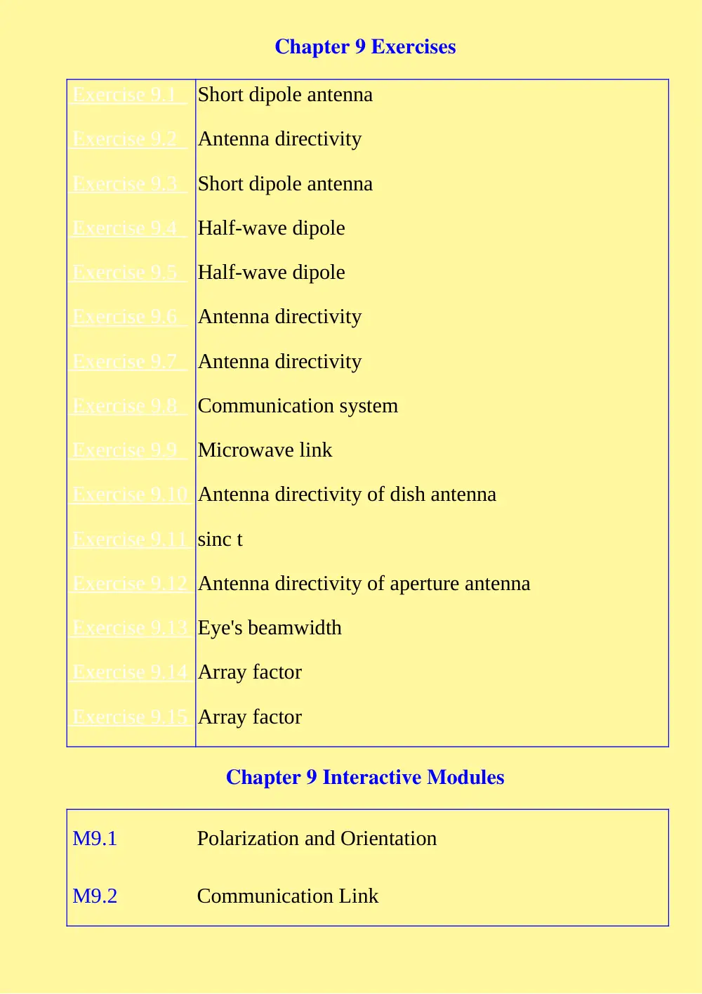Chapter 9 Exercises Exercise 9.1 Short dipole antenna Exercise 9.2 Antenna directivity Exercise 9.3 Short dipole antenna Exercise 9.4 Half-wave dipole Exercise 9.5 Half-wave dipole Exercise 9.6 Antenna directivity Exercise 9.7 Antenna directivity Exercise 9.8 Communication system Exercise 9.9 Microwave link Exercise 9.10 Antenna directivity of dish antenna Exercise 9.11 sinc t Exercise 9.12 Antenna directivity of aperture antenna Exercise 9.13 Eye's beamwidth Exercise 9.14 Array factor Exercise 9.15 Array factor Chapter 9 Interactive Modules M9.1 Polarization and Orientation M9.2 Communication Link 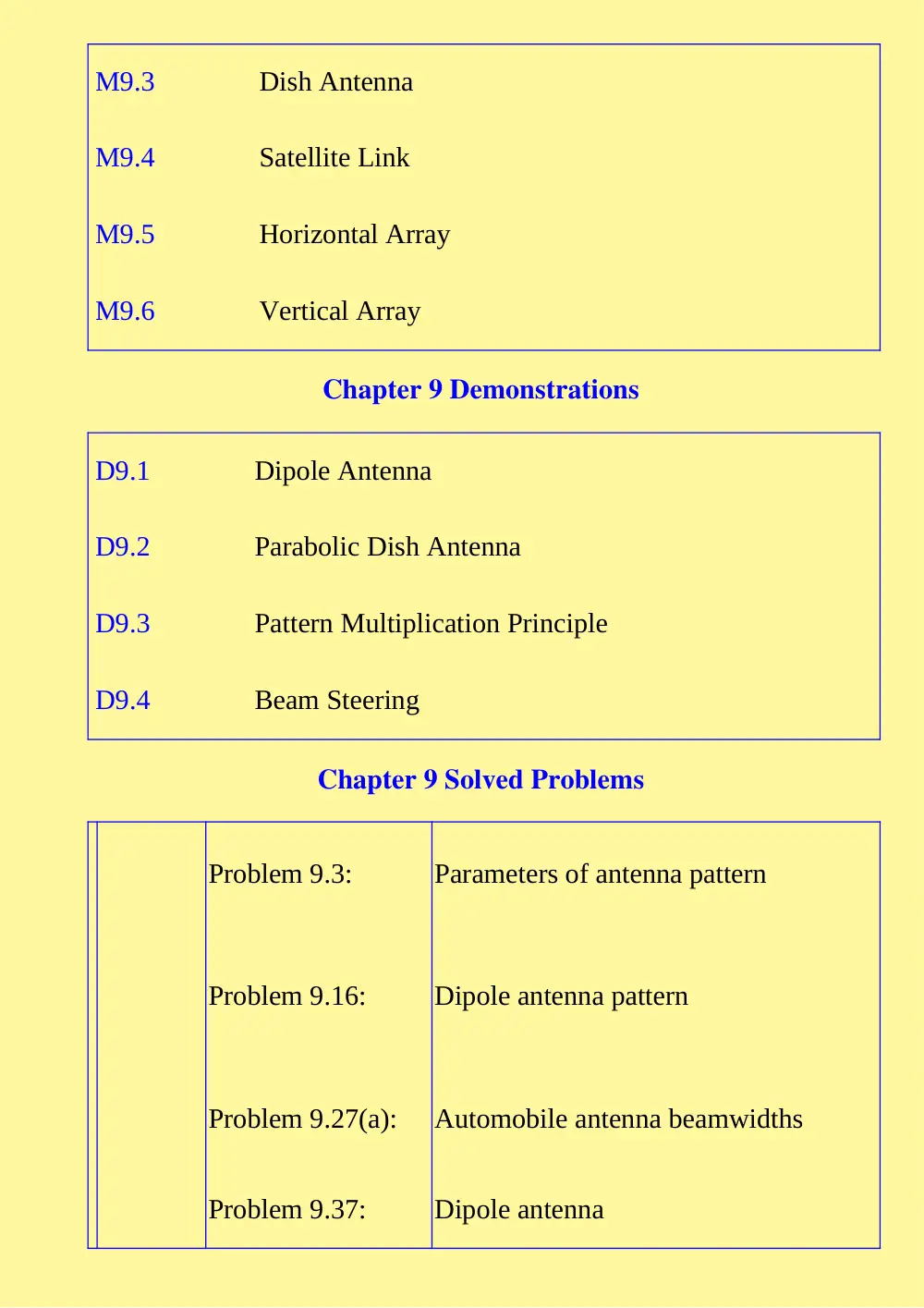M9.3 Dish Antenna M9.4 Satellite Link M9.5 Horizontal Array M9.6 Vertical Array Chapter 9 Demonstrations D9.1 Dipole Antenna D9.2 Parabolic Dish Antenna D9.3 Pattern Multiplication Principle D9.4 Beam Steering Chapter 9 Solved Problems Problem 9.3: Parameters of antenna pattern Problem 9.16: Dipole antenna pattern Problem 9.27(a): Automobile antenna beamwidths Problem 9.37: Dipole antenna Problem 9.38: Communication system Problem 9.39: Half-wave dipole antenna Problem 9.40: Five-element antenna array Antenna Pattern 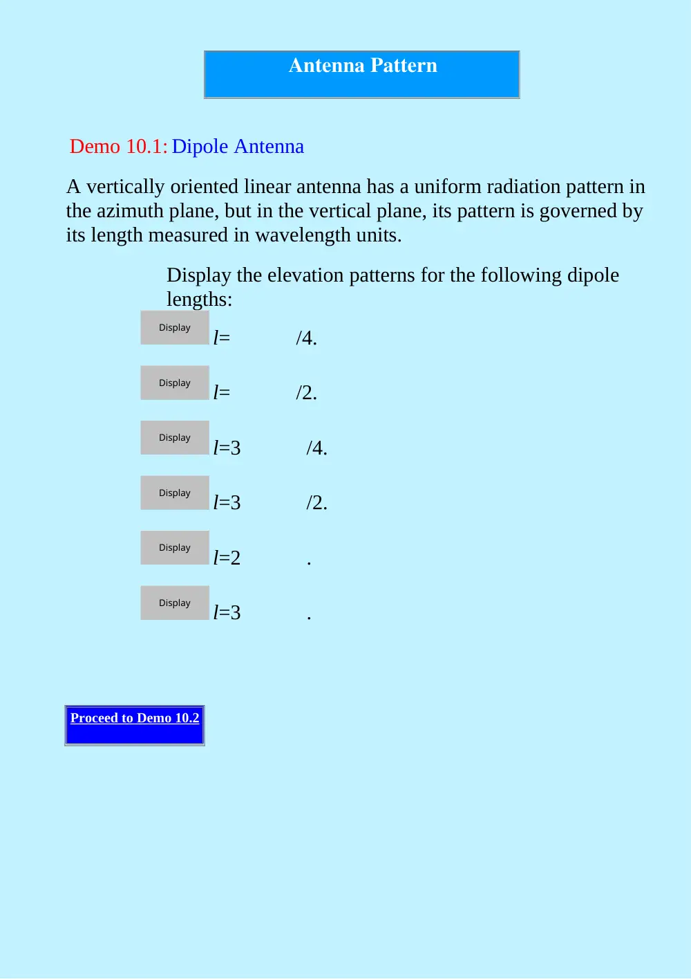Demo 10.1: Dipole Antenna A vertically oriented linear antenna has a uniform radiation pattern in the azimuth plane, but in the vertical plane, its pattern is governed by its length measured in wavelength units. Display the elevation patterns for the following dipole lengths: l= /4. l= /2. l=3 /4. l=3 /2. l=2 . l=3 . 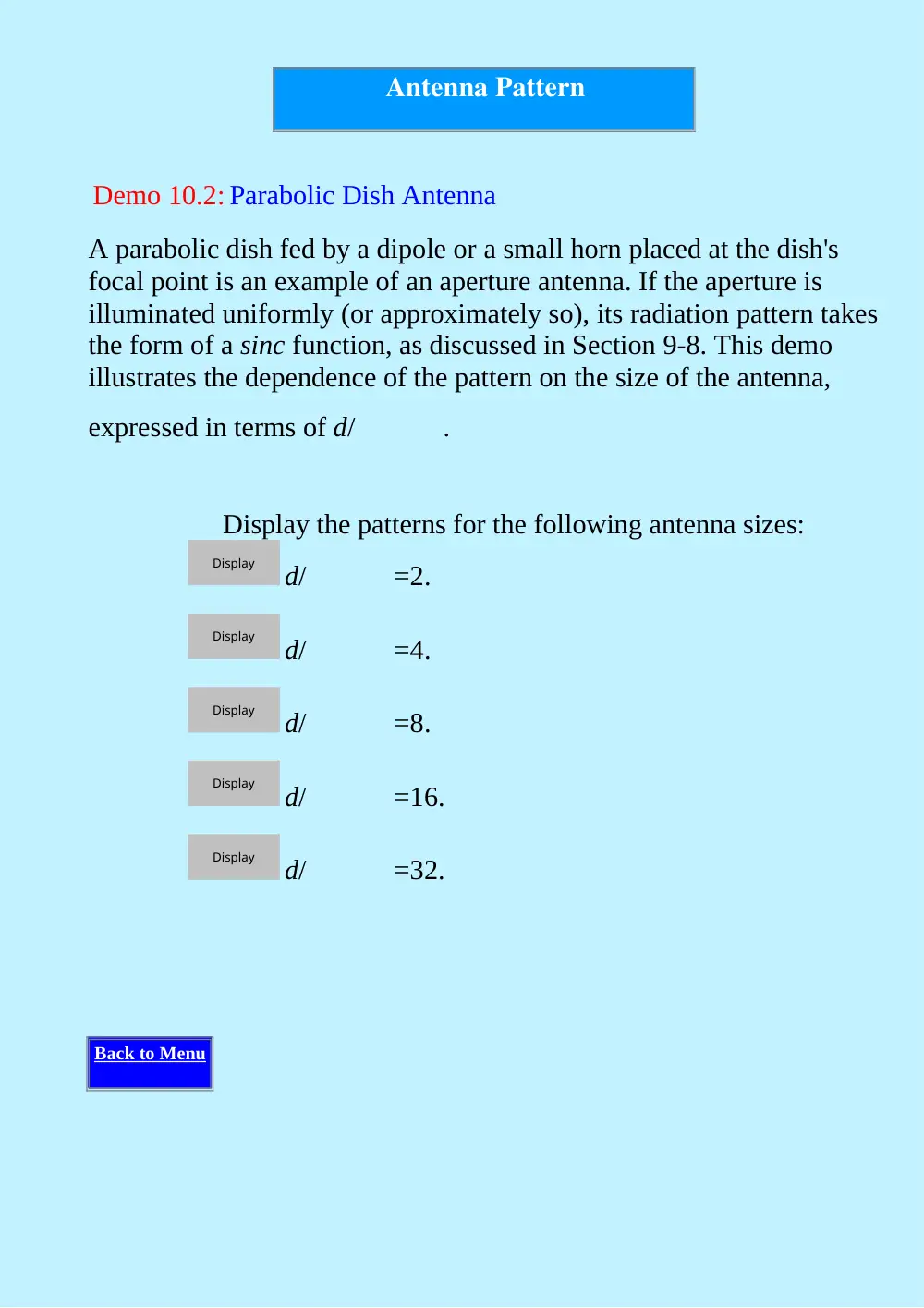Proceed to Demo 10.2 Display Display Display Display Display Display Antenna Pattern Demo 10.2: Parabolic Dish Antenna A parabolic dish fed by a dipole or a small horn placed at the dish's focal point is an example of an aperture antenna. If the aperture is illuminated uniformly (or approximately so), its radiation pattern takes the form of a sinc function, as discussed in Section 9-8. This demo illustrates the dependence of the pattern on the size of the antenna, expressed in terms of d/ . Display the patterns for the following antenna sizes: d/ =2. d/ =4. d/ =8. d/ =16. d/ =32. Back to Menu Display Display Display Display Display Chapter 10 Demonstrations D10.1 Dipole Antenna D10.2 Parabolic Dish Antenna Chapter 10 Exercises Exercise 10.1 Short dipole antenna Exercise 10.2 Antenna directivity Exercise 10.3 Short dipole antenna Exercise 10.4 Half-wave dipole Exercise 10.5 Half-wave dipole Exercise 10.6 Antenna directivity Exercise 10.7 Antenna directivity Exercise 10.8 Communication system Exercise 10.9 Microwave link Exercise 10.10 Antenna directivity of dish antenna One reason that cell towers might not have been designed with circularly polarized antennas is because of polarization mismatch: you are guaranteed not to receive half the tranmitted power when you are sending a signal from a linearly polarized to a circularly polarized antenna. In the case of the cell phone itself, that would increase power consumption and make the whole phone bigger. The reception would be pretty poor. Although he has oriented his cell- phone antenna such that the power transmitted towards the base station is maximized, the polarizations of the transmitting and receiving antennas are orthogonal to one another. Hence, no signal would be intercepted. There would be no reception because both the recieving antenna and transmitting antenna have nulls in their patterns along the dipole axis. Thus, no signal would be received. If you try these experiments you may well discover that you do not get zero reception with different orientations of the phone. This is because we have not considered the effects of the signal bouncing off the ground and other surrounding objects (multipath) and the cross polarization effects that come with that. Although the use of a circularly polarized antenna on the cell-phone tower would solve the polarization mismatch problem with a linearly polarized cell-phone antenna, the cell-phone antenna can intercept no more than half of the circularly polarized power incident upon it. Hence, to maintain the same signal level, it would require the tower antenna to radiate twice as much power as it would with a dipole, and the same is true for the cell-phone antenna when it operates in a transmitting mode. Making both antennas circularly polarized introduces a different set of orientation losses. Dipole Antenna Module 10.1: Polarization and Orientation Given: A cellular phone base station with a vertical dipole antenna at the top, and a cellular phone user nearby. Q1.  Imagine someone in his backyard pool, talking on the phone and sunning himself. His cell phone is oriented such that the antenna is horizontal, as shown in the figure. Is his reception: Q2.  Now consider the same person, who has stood up so that his cell phone is oriented vertically, and moved his location so that he is now directly under the base station antenna, as shown in the figure. Note that the tip of his antenna is pointing directly towards the tip of the base station antenna. Is his reception: Q3.  Why is it that cell-phone towers do not use circularly polarized Good Bad explain Good Bad explain antennas? power consumption/polarization issues mutual impedance/pattern issues Proceed to Module 10.2 select select explain Dipole Antenna Module 10.2: Communication Link Given: A 300-MHz communication system that utilizes vertically oriented half-wavelength long dipoles on both the transmitter and receiver ends of a 10-km link. Q1. How long are the dipole antennas? l= m Q2. Assuming the transmitter source is a sinusoidal voltage generator with 300 V, and assuming that each dipole is tuned to exhibit an approxima impedance of 75 , what is the amplitude of the current exiting dipole antenna? It0= A Q3. What is the average power density of the wave incident upon the recei antenna? Si= W/m2 Q4. What is the corresponding power intercepted by the receiving dipole a Pint= nW Q5. If the receiver circuit is designed to exhibit an equivalent input impeda , so as to match it to the receiving antenna and the in-between what is the amplitude of the current flowing through ZL? check answer help I give up check answer help I give up check answer help I give up check answer help I give up IL0= A Proceed to Module 10.3 check answer help I give up Antenna Properties Module 10.3: Dish Antenna Given: A parabolic dish antenna of diameter d1 operating at frequency f1. Q1. If the antenna is operated at a higher frequency, namely f2=10f1, how will the antenna beamwidth and directivity change? (a) Beamwidth will: Increase by a factor of 10. Increase by a factor of 100. Not change. Decrease by a factor of 10. Decrease by a factor of 100. (b) Directivity will: Increase by a factor of 10. Increase by a factor of 100. Not change. select select select select select explain select select select Decrease by a factor of 10. Decrease by a factor of 100. Q2. If the frequency is increased from f1 to f2=10f1 and simultaneously the antenna is reduced in size to a new diameter d2=d1/10, what will become of the beamwidth and directivity? (a) Beamwidth will: Increase by a factor of 10. Increase by a factor of 100. Not change. Decrease by a factor of 10. Decrease by a factor of 100. (b) Directivity will: Increase by a factor of 10. Increase by a factor of 100. Not change. select select explain select select select select select explain select select select Decrease by a factor of 10. Decrease by a factor of 100. Proceed to Module 10.4 select select explain Communication System Module 10.4: Satellite Link Given: A 6-GHz satellite to Earth communication link. The satellite, at 40,000 km above Earth's surface, transmits 100 W through a lossless 2-m diameter dish antenna. Q1. How large in area is the 3-dB footprint of the satellite beam on the sur Earth? A= x105km2 Q2. What is the power intercepted by a small, ground-based, 15 cm diame antenna pointed toward the satellite? Pint= x10-12W Q3. If the receiver is characterized by a system noise temperature of 100 K receiver bandwidth is 5 MHz, what is the receiver noise power? Pn= x10-15W Q4. What is the receiver signal-to-noise ratio? Sn= dB Back to Menu check answer help I give up check answer help I give up check answer help I give up check answer help I give up Chapter 10 Interactive Modules M10.1 Polarization and Orientation M10.2 Communication Link M10.3 Dish Antenna M10.4 Satellite Link Chapter 10 Solved Problems Problem 10.3: Parameters of antenna pattern Problem 10.20: Dipole antenna Problem 10.21: Communication system Problem 10.22: Half-wave dipole antenna THIS IS THE MAPPING BETWEEN MakeImages IMAGES AND CH3 MODULES/DEMOS: source1/img1a.gif --> ~/ch3/demo3.1a.gifsource1/img1b.gif --> ~/ch3/demo3.1b.gifsource1/img2a.gif --> ~/ch3/demo3.2a.gifsource1/img2b.gif --> ~/ch3/demo3.2b.gifsource1/img3a.gif --> ~/ch3/demo3.3a.gif source1/img3b.gif --> ~/ch3/demo3.3b.gifsource1/img4a.gif --> ~/ch3/demo3.5a.gifsource1/img4b.gif --> ~/ch3/demo3.5b.gifsource1/img5a.gif --> ~/ch3/demo3.6a.gifsource1/img5b.gif --> ~/ch3/demo3.6b.gif source1/img6a.gif --> ~/ch3/demo3.8a.gifsource1/img6b.gif --> ~/ch3/demo3.8b.gifsource1/img7a.gif --> ~/ch3/demo3.7a.gifsource1/img7b.gif --> ~/ch3/demo3.7b.gifsource1/img8a.gif --> ~/ch3/demo3.9a.gif source1/img8b.gif --> ~/ch3/demo3.9b.gifsource1/img9a.gif --> ~/ch3/demo3.4a.gifsource1/img9b.gif --> ~/ch3/demo3.4b.gifsource2/img1a.gif --> ~/ch3/demo3.10b.gifsource2/img1b.gif --> ~/ch3/demo3.10a.gif source2/img2a.gif --> NOT USEDsource2/img2b.gif --> NOT USED source2/img3a.gif --> ~/ch3/demo3.11b.gifsource2/img3b.gif --> ~/ch3/demo3.11a.gifsource2/img4a.gif --> ~/ch3/demo3.14b.gifsource2/img4b.gif --> ~/ch3/demo3.14a.gifsource2/img5a.gif --> ~/ch3/demo3.15b.gif source2/img5b.gif --> ~/ch3/demo3.15a.gifsource2/img6a.gif --> ~/ch3/mod3.7b.gifsource2/img6b.gif --> ~/ch3/mod3.7a.gifsource2/img7a.gif --> ~/ch3/mod3.10b.gifsource2/img7b.gif --> ~/ch3/mod3.10a.gif source2/img8a.gif --> ~/ch3/mod3.9b.gifsource2/img8b.gif --> ~/ch3/mod3.9a.gifsource2/img9a.gif --> ~/ch3/mod3.8b.gifsource2/img9b.gif --> ~/ch3/mod3.8a.gifsource2/img10a.gif --> ~/ch3/mod3.11b.gif source2/img10b.gif --> ~/ch3/mod3.11a.gifsource2/img11a.gif --> ~/ch3/demo3.12b.gifsource2/img11b.gif --> ~/ch3/demo3.12a.gif source2/img12a.gif --> ~/ch3/demo3.13b.gifsource2/img12b.gif --> ~/ch3/demo3.13a.gif Chapter 3 Exercises Exercise 3.1 Distance vector Exercise 3.2 Vector algebra Exercise 3.3 Vector algebra Exercise 3.4 Cylinder volume Exercise 3.5 Coordinate transformation Exercise 3.6 Coordinate transformation Exercise 3.7 Gradient Exercise 3.8 Directional derivative Exercise 3.9 Divergence in cartesian cooordinates Exercise 3.10 Divergence in cylindrical cooordinates Exercise 3.11 Flux through a surface Exercise 3.12 Divergence theorem Exercise 3.13 Curl in cylindrical coordinates Exercise 3.14 Curl in spherical coordinates Chapter 3 Interactive Modules M3.1 Two Parallel Vectors M3.2 Two Intersecting Vectors M3.3 Intersecting Vectors 2 M3.4 Dot Product M3.5 Shining Star M3.6 Sea-Land Temperature Profile M3.7 Divergence of M3.8 Divergence of M3.9 Divergence of M3.10 Divergence of M3.11 Divergence of Chapter 3 Demonstrations Gradient of Scalar Fields D3.1 D3.2 D3.3 D3.4 D3.5 D3.6 D3.7 D3.8 D3.9 Divergence of Vector Fields D3.10 D3.11 D3.12 D3.13 D3.14 D3.15 Chapter 3 Solved Problems Problem 3.9: Unit vector Problem 3.17(b,e): Sketching vector fields Problem 3.19(a): Converting coordinates from cartesian to cylindrical and spherical Problem 3.21(b):  Converting coordinates from spherical to cylindrical Problem 3.22(d):  Surface area Problem 3.31(c): Transform vectors to spherical coordinates Problem 3.32(d):  Calculating the gradient Problem 3.41: Verify the divergence theorem Problem 3.45: Verify Stokes's theorem Problem 3.50: Vector algebra Problem 3.51: Vector algebra Problem 3.52: Vector orthogonality Problem 3.53: Vector transformation Problem 3.54: Line integral Problem 3.55: Stokes's theorem Problem 3.56: Laplacian Gradient of Scalar Fields Demo 3.1: Gradient of Scalar Fields Given: A scalar field defined by: The field T is displayed graphically in the figure, wherein the brightness of the image at a given location is proportional to the magnitude of T at that location. the graphical and analytical solution for T Proceed to Demo 3.2 Display Divergence of Vector Fields Demo 3.10: Divergence of Vector Fields Given: A vector field defined by: The vector A is displayed graphically in the figure, wherein vectors are used to depict the direction and magnitude of A at any given location. the graphical and analytical solution for . A Proceed to Demo 3.11 Display Divergence of Vector Fields Demo 3.11: Divergence of Vector Fields Given: A vector field defined by: The vector A is displayed graphically in the figure, wherein vectors are used to depict the direction and magnitude of A at any given location. the graphical and analytical solution for . A Proceed to Demo 3.12 Display Divergence of Vector Fields Demo 3.12: Divergence of Vector Fields Given: A vector field defined by: The vector A is displayed graphically in the figure, wherein vectors are used to depict the direction and magnitude of A at any given location. the graphical and analytical solution for . A Proceed to Demo 3.13 Display Divergence of Vector Fields Demo 3.13: Divergence of Vector Fields Given: A vector field defined by: The vector A is displayed graphically in the figure, wherein vectors are used to depict the direction and magnitude of A at any given location. the graphical and analytical solution for . A Proceed to Demo 3.14 Display Divergence of Vector Fields Demo 3.14: Divergence of Vector Fields Given: A vector field defined by: The vector A is displayed graphically in the figure, wherein vectors are used to depict the direction and magnitude of A at any given location. the graphical and analytical solution for . A Proceed to Demo 3.15 Display Divergence of Vector Fields Demo 3.15: Divergence of Vector Fields Given: A vector field defined by: The vector A is displayed graphically in the figure, wherein vectors are used to depict the direction and magnitude of A at any given location. the graphical and analytical solution for . A Back to Menu Display Gradient of Scalar Fields Demo 3.2: Gradient of Scalar Fields Given: A scalar field defined by: The field T is displayed graphically in the figure, wherein the brightness of the image at a given location is proportional to the magnitude of T at that location. the graphical and analytical solution for T Proceed to Demo 3.3 Display Gradient of Scalar Fields Demo 3.3: Gradient of Scalar Fields Given: A scalar field defined by: The field T is displayed graphically in the figure, wherein the brightness of the image at a given location is proportional to the magnitude of T at that location. the graphical and analytical solution for T Proceed to Demo 3.4 Display Gradient of Scalar Fields Demo 3.4: Gradient of Scalar Fields Given: A scalar field defined by: The field T is displayed graphically in the figure, wherein the brightness of the image at a given location is proportional to the magnitude of T at that location. the graphical and analytical solution for T Proceed to Demo 3.5 Display Gradient of Scalar Fields Demo 3.5: Gradient of Scalar Fields Given: A scalar field defined by: The field T is displayed graphically in the figure, wherein the brightness of the image at a given location is proportional to the magnitude of T at that location. the graphical and analytical solution for T Proceed to Demo 3.6 Display Gradient of Scalar Fields Demo 3.6: Gradient of Scalar Fields Given: A scalar field defined by: The field T is displayed graphically in the figure, wherein the brightness of the image at a given location is proportional to the magnitude of T at that location. the graphical and analytical solution for T Proceed to Demo 3.7 Display Gradient of Scalar Fields Demo 3.7 Gradient of Scalar Fields Given: A scalar field defined by: The field T is displayed graphically in the figure, wherein the brightness of the image at a given location is proportional to the magnitude of T at that location. the graphical and analytical solution for T Proceed to Demo 3.8 Display