FINA 210 Problems Solution Manual 9th Ed, Spring 2011

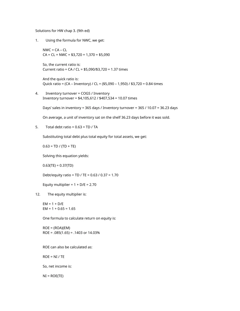
Solutions for HW chap 3. (9th ed) 1.        Using the formula for NWC, we get: NWC = CA – CL CA = CL + NWC = $3,720 + 1,370 = $5,090 So, the current ratio is: Current ratio = CA / CL = $5,090/$3,720 = 1.37 times And the quick ratio is: Quick ratio = (CA – Inventory) / CL = ($5,090 – 1,950) / $3,720 = 0.84 times 4.        Inventory turnover = COGS / Inventory Inventory turnover = $4,105,612 / $407,534 = 10.07 times Days’ sales in inventory = 365 days / Inventory turnover = 365 / 10.07 = 36.23 days On average, a unit of inventory sat on the shelf 36.23 days before it was sold. 5.        Total debt ratio = 0.63 = TD / TA Substituting total debt plus total equity for total assets, we get: 0.63 = TD / (TD + TE) Solving this equation yields: 0.63(TE) = 0.37(TD) Debt/equity ratio = TD / TE = 0.63 / 0.37 = 1.70 Equity multiplier = 1 + D/E = 2.70 12.        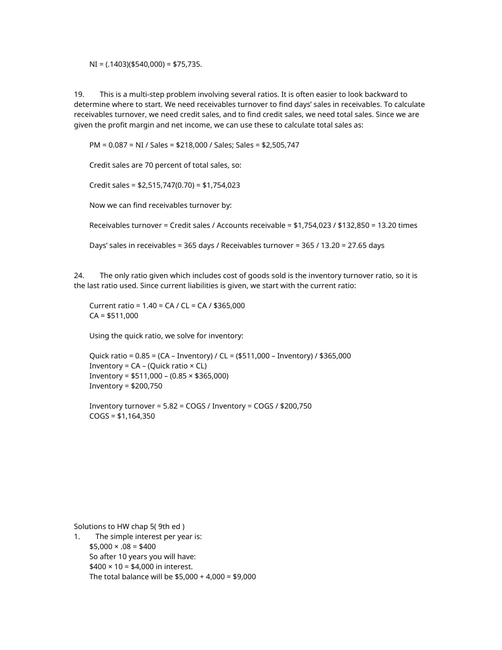The equity multiplier is: EM = 1 + D/E EM = 1 + 0.65 = 1.65 One formula to calculate return on equity is: ROE = (ROA)(EM) ROE = .085(1.65) = .1403 or 14.03% ROE can also be calculated as: ROE = NI / TE So, net income is: NI = ROE(TE) NI = (.1403)($540,000) = $75,735. 19.        This is a multi-step problem involving several ratios. It is often easier to look backward to determine where to start. We need receivables turnover to find days’ sales in receivables. To calculate receivables turnover, we need credit sales, and to find credit sales, we need total sales. Since we are given the profit margin and net income, we can use these to calculate total sales as: PM = 0.087 = NI / Sales = $218,000 / Sales; Sales = $2,505,747 Credit sales are 70 percent of total sales, so: Credit sales = $2,515,747(0.70) = $1,754,023 Now we can find receivables turnover by: Receivables turnover = Credit sales / Accounts receivable = $1,754,023 / $132,850 = 13.20 times Days’ sales in receivables = 365 days / Receivables turnover = 365 / 13.20 = 27.65 days 24.        The only ratio given which includes cost of goods sold is the inventory turnover ratio, so it is the last ratio used. Since current liabilities is given, we start with the current ratio: Current ratio = 1.40 = CA / CL = CA / $365,000 CA = $511,000 Using the quick ratio, we solve for inventory: Quick ratio = 0.85 = (CA – Inventory) / CL = ($511,000 – Inventory) / $365,000 Inventory = CA – (Quick ratio × CL) Inventory = $511,000 – (0.85 × $365,000) Inventory = $200,750 Inventory turnover = 5.82 = COGS / Inventory = COGS / $200,750 COGS = $1,164,350 Solutions to HW chap 5( 9th ed ) 1.        The simple interest per year is: $5,000 × .08 = $400 So after 10 years you will have: $400 × 10 = $4,000 in interest. 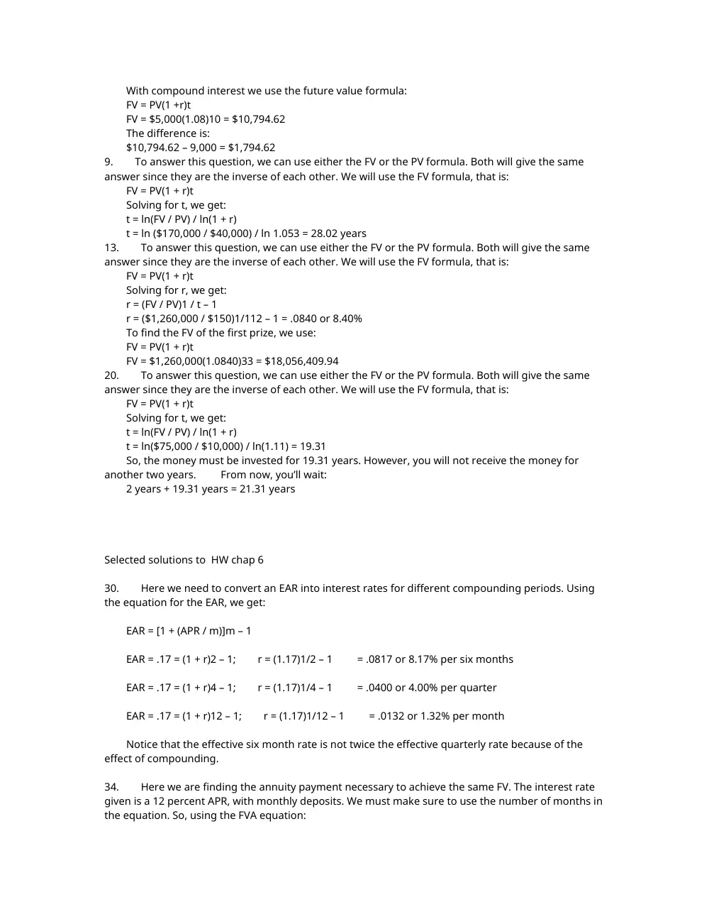The total balance will be $5,000 + 4,000 = $9,000 With compound interest we use the future value formula: FV = PV(1 +r)t FV = $5,000(1.08)10 = $10,794.62 The difference is: $10,794.62 – 9,000 = $1,794.62 9.        To answer this question, we can use either the FV or the PV formula. Both will give the same answer since they are the inverse of each other. We will use the FV formula, that is: FV = PV(1 + r)t Solving for t, we get: t = ln(FV / PV) / ln(1 + r) t = ln ($170,000 / $40,000) / ln 1.053 = 28.02 years 13.        To answer this question, we can use either the FV or the PV formula. Both will give the same answer since they are the inverse of each other. We will use the FV formula, that is: FV = PV(1 + r)t Solving for r, we get: r = (FV / PV)1 / t – 1 r = ($1,260,000 / $150)1/112 – 1 = .0840 or 8.40% To find the FV of the first prize, we use: FV = PV(1 + r)t FV = $1,260,000(1.0840)33 = $18,056,409.94 20.        To answer this question, we can use either the FV or the PV formula. Both will give the same answer since they are the inverse of each other. We will use the FV formula, that is: FV = PV(1 + r)t Solving for t, we get: t = ln(FV / PV) / ln(1 + r) t = ln($75,000 / $10,000) / ln(1.11) = 19.31 So, the money must be invested for 19.31 years. However, you will not receive the money for another two years.         From now, you’ll wait: 2 years + 19.31 years = 21.31 years Selected solutions to  HW chap 6 30.        Here we need to convert an EAR into interest rates for different compounding periods. Using the equation for the EAR, we get: EAR = [1 + (APR / m)]m – 1 EAR = .17 = (1 + r)2 – 1;        r = (1.17)1/2 – 1         = .0817 or 8.17% per six months EAR = .17 = (1 + r)4 – 1;        r = (1.17)1/4 – 1         = .0400 or 4.00% per quarter EAR = .17 = (1 + r)12 – 1;        r = (1.17)1/12 – 1         = .0132 or 1.32% per month Notice that the effective six month rate is not twice the effective quarterly rate because of the effect of compounding. 34.        Here we are finding the annuity payment necessary to achieve the same FV. The interest rate given is a 12 percent APR, with monthly deposits. We must make sure to use the number of months in the equation. So, using the FVA equation: Starting today: FVA = C[{[1 + (.12/12) ]480 – 1} / (.12/12)] C = $1,000,000 / 11,764.77 = $85.00 Starting in 10 years: FVA = C[{[1 + (.12/12) ]360 – 1} / (.12/12)] C = $1,000,000 / 3,494.96 = $286.13 Starting in 20 years: FVA = C[{[1 + (.12/12) ]240 – 1} / (.12/12)] C = $1,000,000 / 989.255 = $1,010.86 Notice that a deposit for half the length of time, i.e. 20 years versus 40 years, does not mean that the annuity payment is doubled. In this example, by reducing the savings period by one-half, the deposit necessary to achieve the same ending value is about twelve times as large. 38.        Since your salary grows at 4 percent per year, your salary next year will be: Next year’s salary = $50,000 (1 + .04) Next year’s salary = $52,000 This means your deposit next year will be: Next year’s deposit = $52,000(.05) Next year’s deposit = $2,600 Since your salary grows at 4 percent, you deposit will also grow at 4 percent. We can use the present value of a growing perpetuity equation to find the value of your deposits today. Doing so, we find: PV = C {[1/(r – g)] – [1/(r – g)] × [(1 + g)/(1 + r)]t} PV = $2,600{[1/(.11 – .04)] – [1/(.11 – .04)] × [(1 + .04)/(1 + .11)]40} PV = $34,399.45 Now, we can find the future value of this lump sum in 40 years. We find: FV = PV(1 + r)t FV = $34,366.45(1 + .11)40 FV = $2,235,994.31 This is the value of your savings in 40 years. 44.        To solve this problem, we simply need to find the PV of each lump sum and add them together. It is important to note that the first cash flow of $1 million occurs today, so we do not need to discount that cash flow. 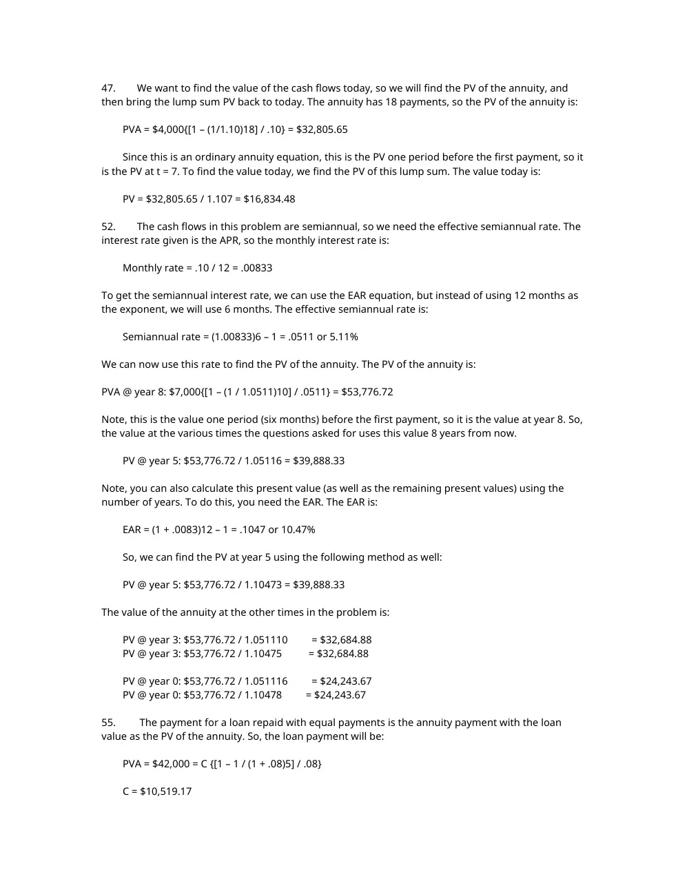The PV of the lottery winnings is: PV = $1,000,000 + $1,500,000/1.09 + $2,000,000/1.092 + $2,500,000/1.093 + $3,000,000/1.094 + $3,500,000/1.095 + $4,000,000/1.096 + $4,500,000/1.097 + $5,000,000/1.098 + $5,500,000/1.099 + $6,000,000/1.0910 PV = $22,812,873.40 47.        We want to find the value of the cash flows today, so we will find the PV of the annuity, and then bring the lump sum PV back to today. The annuity has 18 payments, so the PV of the annuity is: PVA = $4,000{[1 – (1/1.10)18] / .10} = $32,805.65 Since this is an ordinary annuity equation, this is the PV one period before the first payment, so it is the PV at t = 7. To find the value today, we find the PV of this lump sum. The value today is: PV = $32,805.65 / 1.107 = $16,834.48 52.        The cash flows in this problem are semiannual, so we need the effective semiannual rate. The interest rate given is the APR, so the monthly interest rate is: Monthly rate = .10 / 12 = .00833 To get the semiannual interest rate, we can use the EAR equation, but instead of using 12 months as the exponent, we will use 6 months. The effective semiannual rate is: Semiannual rate = (1.00833)6 – 1 = .0511 or 5.11% We can now use this rate to find the PV of the annuity. The PV of the annuity is: PVA @ year 8: $7,000{[1 – (1 / 1.0511)10] / .0511} = $53,776.72 Note, this is the value one period (six months) before the first payment, so it is the value at year 8. So, the value at the various times the questions asked for uses this value 8 years from now. PV @ year 5: $53,776.72 / 1.05116 = $39,888.33 Note, you can also calculate this present value (as well as the remaining present values) using the number of years. To do this, you need the EAR. The EAR is: EAR = (1 + .0083)12 – 1 = .1047 or 10.47% So, we can find the PV at year 5 using the following method as well: PV @ year 5: $53,776.72 / 1.10473 = $39,888.33 The value of the annuity at the other times in the problem is: PV @ year 3: $53,776.72 / 1.051110         = $32,684.88 PV @ year 3: $53,776.72 / 1.10475          = $32,684.88 PV @ year 0: $53,776.72 / 1.051116         = $24,243.67 PV @ year 0: $53,776.72 / 1.10478         = $24,243.67 55.         The payment for a loan repaid with equal payments is the annuity payment with the loan value as the PV of the annuity. 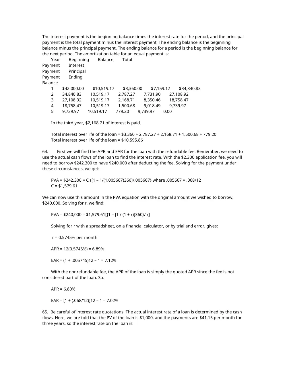So, the loan payment will be: PVA = $42,000 = C {[1 – 1 / (1 + .08)5] / .08} C = $10,519.17 The interest payment is the beginning balance times the interest rate for the period, and the principal payment is the total payment minus the interest payment. The ending balance is the beginning balance minus the principal payment. The ending balance for a period is the beginning balance for the next period. The amortization table for an equal payment is: Year        Beginning        Balance        Total Payment        Interest Payment        Principal Payment        Ending Balance 1        $42,000.00        $10,519.17        $3,360.00        $7,159.17        $34,840.83 2        34,840.83        10,519.17        2,787.27        7,731.90        27,108.92 3        27,108.92        10,519.17        2,168.71        8,350.46        18,758.47 4        18,758.47        10,519.17        1,500.68        9,018.49        9,739.97 5        9,739.97        10,519.17        779.20        9,739.97        0.00 In the third year, $2,168.71 of interest is paid. Total interest over life of the loan = $3,360 + 2,787.27 + 2,168.71 + 1,500.68 + 779.20 Total interest over life of the loan = $10,595.86 64.        First we will find the APR and EAR for the loan with the refundable fee. Remember, we need to use the actual cash flows of the loan to find the interest rate. With the $2,300 application fee, you will need to borrow $242,300 to have $240,000 after deducting the fee. Solving for the payment under these circumstances, we get: PVA = $242,300 = C {[1 – 1/(1.005667)360]/.005667} where .005667 = .068/12 C = $1,579.61 We can now use this amount in the PVA equation with the original amount we wished to borrow, $240,000. Solving for r, we find: PVA = $240,000 = $1,579.61[{1 – [1 / (1 + r)]360}/ r] Solving for r with a spreadsheet, on a financial calculator, or by trial and error, gives: r = 0.5745% per month APR = 12(0.5745%) = 6.89% EAR = (1 + .005745)12 – 1 = 7.12% With the nonrefundable fee, the APR of the loan is simply the quoted APR since the fee is not considered part of the loan. So: APR = 6.80% EAR = [1 + (.068/12)]12 – 1 = 7.02% 65.  Be careful of interest rate quotations. The actual interest rate of a loan is determined by the cash flows. 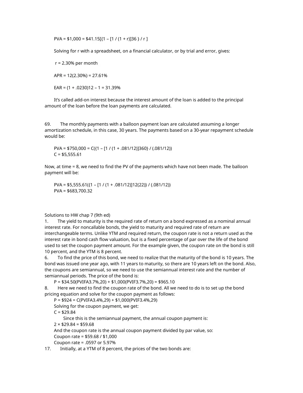Here, we are told that the PV of the loan is $1,000, and the payments are $41.15 per month for three years, so the interest rate on the loan is: PVA = $1,000 = $41.15[{1 – [1 / (1 + r)]36 } / r ] Solving for r with a spreadsheet, on a financial calculator, or by trial and error, gives: r = 2.30% per month APR = 12(2.30%) = 27.61% EAR = (1 + .0230)12 – 1 = 31.39% It’s called add-on interest because the interest amount of the loan is added to the principal amount of the loan before the loan payments are calculated. 69.        The monthly payments with a balloon payment loan are calculated assuming a longer amortization schedule, in this case, 30 years. The payments based on a 30-year repayment schedule would be: PVA = $750,000 = C({1 – [1 / (1 + .081/12)]360} / (.081/12)) C = $5,555.61 Now, at time = 8, we need to find the PV of the payments which have not been made. The balloon payment will be: PVA = $5,555.61({1 – [1 / (1 + .081/12)]12(22)} / (.081/12)) PVA = $683,700.32 Solutions to HW chap 7 (9th ed) 1.        The yield to maturity is the required rate of return on a bond expressed as a nominal annual interest rate. For noncallable bonds, the yield to maturity and required rate of return are interchangeable terms. Unlike YTM and required return, the coupon rate is not a return used as the interest rate in bond cash flow valuation, but is a fixed percentage of par over the life of the bond used to set the coupon payment amount. For the example given, the coupon rate on the bond is still 10 percent, and the YTM is 8 percent. 6.        To find the price of this bond, we need to realize that the maturity of the bond is 10 years. The bond was issued one year ago, with 11 years to maturity, so there are 10 years left on the bond. Also, the coupons are semiannual, so we need to use the semiannual interest rate and the number of semiannual periods. The price of the bond is: P = $34.50(PVIFA3.7%,20) + $1,000(PVIF3.7%,20) = $965.10 8.        Here we need to find the coupon rate of the bond. All we need to do is to set up the bond pricing equation and solve for the coupon payment as follows: P = $924 = C(PVIFA3.4%,29) + $1,000(PVIF3.4%,29) Solving for the coupon payment, we get: C = $29.84 Since this is the semiannual payment, the annual coupon payment is: 2 × $29.84 = $59.68 And the coupon rate is the annual coupon payment divided by par value, so: Coupon rate = $59.68 / $1,000 Coupon rate = .0597 or 5.97% 17.        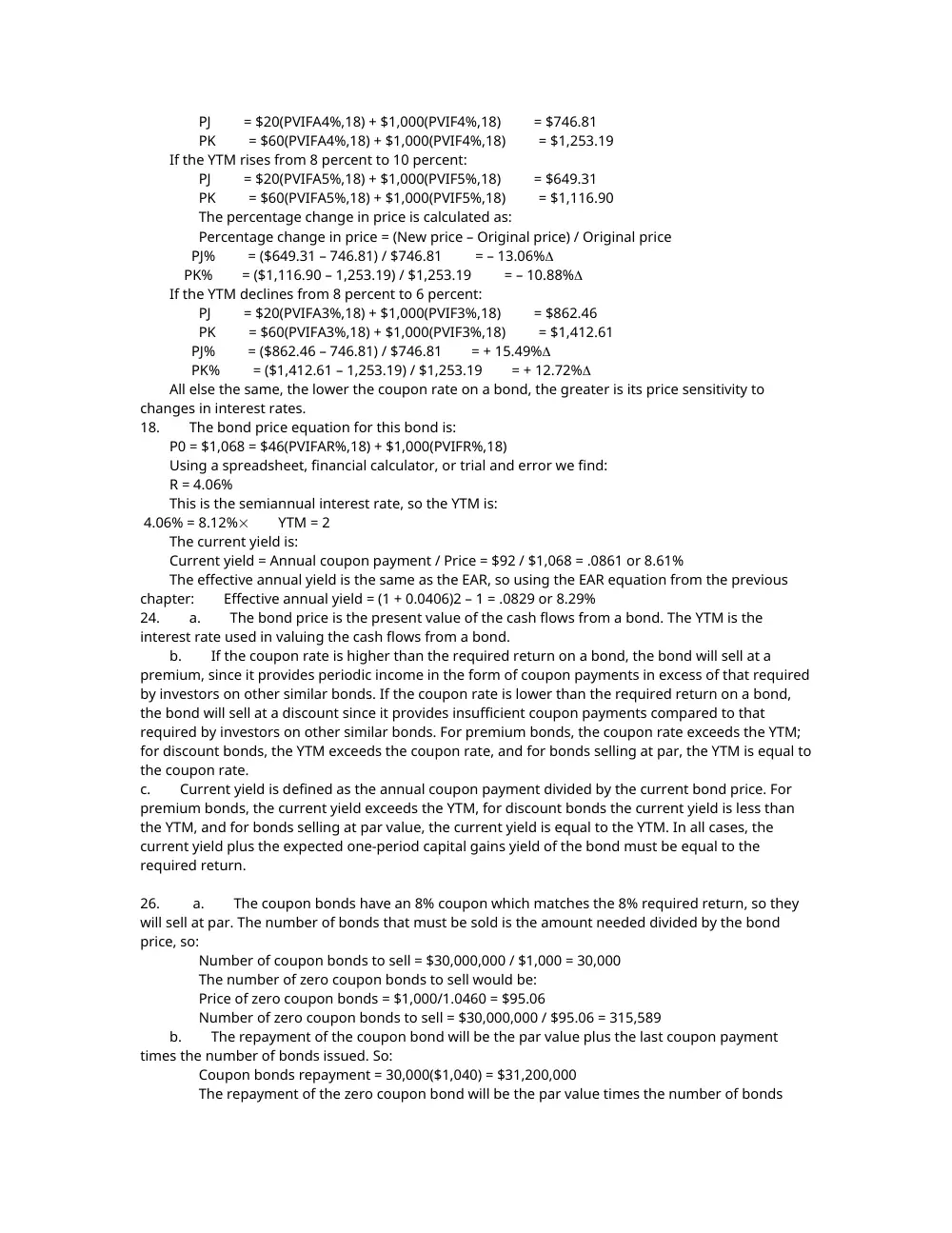Initially, at a YTM of 8 percent, the prices of the two bonds are: PJ         = $20(PVIFA4%,18) + $1,000(PVIF4%,18)         = $746.81 PK         = $60(PVIFA4%,18) + $1,000(PVIF4%,18)         = $1,253.19 If the YTM rises from 8 percent to 10 percent: PJ         = $20(PVIFA5%,18) + $1,000(PVIF5%,18)         = $649.31 PK         = $60(PVIFA5%,18) + $1,000(PVIF5%,18)         = $1,116.90 The percentage change in price is calculated as: Percentage change in price = (New price – Original price) / Original price PJ%         = ($649.31 – 746.81) / $746.81         = – 13.06% PK%        = ($1,116.90 – 1,253.19) / $1,253.19         = – 10.88% If the YTM declines from 8 percent to 6 percent: PJ         = $20(PVIFA3%,18) + $1,000(PVIF3%,18)         = $862.46 PK         = $60(PVIFA3%,18) + $1,000(PVIF3%,18)         = $1,412.61 PJ%         = ($862.46 – 746.81) / $746.81        = + 15.49% PK%         = ($1,412.61 – 1,253.19) / $1,253.19        = + 12.72% All else the same, the lower the coupon rate on a bond, the greater is its price sensitivity to changes in interest rates. 18.        The bond price equation for this bond is: P0 = $1,068 = $46(PVIFAR%,18) + $1,000(PVIFR%,18) Using a spreadsheet, financial calculator, or trial and error we find: R = 4.06% This is the semiannual interest rate, so the YTM is: 4.06% = 8.12%        YTM = 2 The current yield is: Current yield = Annual coupon payment / Price = $92 / $1,068 = .0861 or 8.61% The effective annual yield is the same as the EAR, so using the EAR equation from the previous chapter:        Effective annual yield = (1 + 0.0406)2 – 1 = .0829 or 8.29% 24.        a.        The bond price is the present value of the cash flows from a bond. The YTM is the interest rate used in valuing the cash flows from a bond. b.        If the coupon rate is higher than the required return on a bond, the bond will sell at a premium, since it provides periodic income in the form of coupon payments in excess of that required by investors on other similar bonds. If the coupon rate is lower than the required return on a bond, the bond will sell at a discount since it provides insufficient coupon payments compared to that required by investors on other similar bonds. For premium bonds, the coupon rate exceeds the YTM; for discount bonds, the YTM exceeds the coupon rate, and for bonds selling at par, the YTM is equal to the coupon rate. c.        Current yield is defined as the annual coupon payment divided by the current bond price. For premium bonds, the current yield exceeds the YTM, for discount bonds the current yield is less than the YTM, and for bonds selling at par value, the current yield is equal to the YTM. In all cases, the current yield plus the expected one-period capital gains yield of the bond must be equal to the required return. 26.         a.        The coupon bonds have an 8% coupon which matches the 8% required return, so they will sell at par. The number of bonds that must be sold is the amount needed divided by the bond price, so: Number of coupon bonds to sell = $30,000,000 / $1,000 = 30,000 The number of zero coupon bonds to sell would be: Price of zero coupon bonds = $1,000/1.0460 = $95.06 Number of zero coupon bonds to sell = $30,000,000 / $95.06 = 315,589 b.        The repayment of the coupon bond will be the par value plus the last coupon payment times the number of bonds issued. So: Coupon bonds repayment = 30,000($1,040) = $31,200,000 The repayment of the zero coupon bond will be the par value times the number of bonds issued, so: Zeroes: repayment = 315,589($1,000) = $315,588,822 27.        We found the maturity of a bond in Problem 22. However, in this case, the maturity is indeterminate. A bond selling at par can have any length of maturity. In other words, when we solve the bond pricing equation as we did in Problem 22, the number of periods can be any positive number. Challenge 29.        To find the capital gains yield and the current yield, we need to find the price of the bond. The current price of Bond P and the price of Bond P in one year is: P:        P0 = $120(PVIFA7%,5) + $1,000(PVIF7%,5) = $1,116.69 P1 = $120(PVIFA7%,4) + $1,000(PVIF7%,4) = $1,097.19 Current yield = $120 / $1,116.69 = .1075 or 10.75% The capital gains yield is: Capital gains yield = (New price – Original price) / Original price Capital gains yield = ($1,097.19 – 1,111.69) / $1,116.69 = –.0175 or –1.75% The current price of Bond D and the price of Bond D in one year is: D:        P0 = $60(PVIFA7%,5) + $1,000(PVIF7%,5) = $883.31 P1 = $60(PVIFA7%,4) + $1,000(PVIF7%,4) = $902.81 Current yield = $60 / $883.81 = .0679 or 6.79% Capital gains yield = ($902.81 – 883.31) / $883.31 = +.0221 or +2.21% All else held constant, premium bonds pay high current income while having price depreciation as maturity nears; discount bonds do not pay high current income but have price appreciation as maturity nears. For either bond, the total return is still 9%, but this return is distributed differently between current income and capital gains. 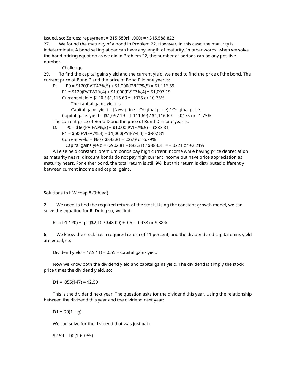Solutions to HW chap 8 (9th ed) 2.        We need to find the required return of the stock. Using the constant growth model, we can solve the equation for R. Doing so, we find: R = (D1 / P0) + g = ($2.10 / $48.00) + .05 = .0938 or 9.38% 6.        We know the stock has a required return of 11 percent, and the dividend and capital gains yield are equal, so: Dividend yield = 1/2(.11) = .055 = Capital gains yield Now we know both the dividend yield and capital gains yield. The dividend is simply the stock price times the dividend yield, so: D1 = .055($47) = $2.59 This is the dividend next year. The question asks for the dividend this year. Using the relationship between the dividend this year and the dividend next year: D1 = D0(1 + g) We can solve for the dividend that was just paid: $2.59 = D0(1 + .055) D0 = $2.59 / 1.055 = $2.45 11.        Here we have a stock that pays no dividends for 10 years. Once the stock begins paying dividends, it will have a constant growth rate of dividends. We can use the constant growth model at that point. It is important to remember that general constant dividend growth formula is: Pt = [Dt × (1 + g)] / (R – g) This means that since we will use the dividend in Year 10, we will be finding the stock price in Year 9. The dividend growth model is similar to the PVA and the PV of a perpetuity: The equation gives you the PV one period before the first payment. So, the price of the stock in Year 9 will be: P9 = D10 / (R – g) = $10.00 / (.14 – .05) = $111.11 The price of the stock today is simply the PV of the stock price in the future. We simply discount the future stock price at the required return. The price of the stock today will be: P0 = $111.11 / 1.149 = $34.17 13.        With supernormal dividends, we find the price of the stock when the dividends level off at a constant growth rate, and then find the PV of the future stock price, plus the PV of all dividends during the supernormal growth period. The stock begins constant growth in Year 4, so we can find the price of the stock in Year 4, at the beginning of the constant dividend growth, as: P4 = D4 (1 + g) / (R – g) = $2.00(1.05) / (.12 – .05) = $30.00 The price of the stock today is the PV of the first four dividends, plus the PV of the Year 3 stock price. So, the price of the stock today will be: P0 = $11.00 / 1.12 + $8.00 / 1.122 + $5.00 / 1.123 + $2.00 / 1.124 + $30.00 / 1.124 = $40.09 17.        We are given the stock price, the dividend growth rate, and the required return, and are asked to find the dividend. Using the constant dividend growth model, we get: P0 = $64 = D0 (1 + g) / (R – g) Solving this equation for the dividend gives us: D0 = $64(.10 – .045) / (1.045) D0 = $3.37 20.        We can use the two-stage dividend growth model for this problem, which is: P0 = [D0(1 + g1)/(R – g1)]{1 – [(1 + g1)/(1 + R)]T}+ [(1 + g1)/(1 + R)]T[D0(1 + g2)/(R – g2)] P0 = [$1.25(1.28)/(.13 – .28)][1 – (1.28/1.13)8] + [(1.28)/(1.13)]8[$1.25(1.06)/(.13 – .06)] P0 = $69.55 Solutions to HW chap 9 (new ed) 7.        The IRR is the interest rate that makes the NPV of the project equal to zero. So, the equation that defines the IRR for this project is: 0 = – $34,000 + $16,000/(1+IRR) + $18,000/(1+IRR)2 + $15,000/(1+IRR)3 Using a spreadsheet, financial calculator, or trial and error to find the root of the equation, we find that: IRR = 20.97% Since the IRR is greater than the required return we would accept the project. 8.        The NPV of a project is the PV of the outflows minus the PV of the inflows. The equation for the NPV of this project at an 11 percent required return is: NPV = – $34,000 + $16,000/1.11 + $18,000/1.112 + $15,000/1.113 = $5,991.49 At an 11 percent required return, the NPV is positive, so we would accept the project. The equation for the NPV of the project at a 30 percent required return is: NPV = – $34,000 + $16,000/1.30 + $18,000/1.302 + $15,000/1.303 = –$4,213.93 At a 30 percent required return, the NPV is negative, so we would reject the project. And the NPV at a 30 percent required return is: NPV        = –$19,500 + $9,800/1.3 + $10,300/1.32 + $8,600/1.33 = –$1,952.44 Notice that as the required return increases, the NPV of the project decreases. This will always be true for projects with conventional cash flows. Conventional cash flows are negative at the beginning of the project and positive throughout the rest of the project. 13.        The IRR is the interest rate that makes the NPV of the project equal to zero. The equation to calculate the IRR of Project X is: 0 = –$15,000 + $8,150/(1+IRR) + $5,050/(1+IRR)2 + $6,800/(1+IRR)3 Using a spreadsheet, financial calculator, or trial and error to find the root of the equation, we find that: IRR = 16.57% For Project Y, the equation to find the IRR is: 0 = –$15,000 + $7,700/(1+IRR) + $5,150/(1+IRR)2 + $7,250/(1+IRR)3 Using a spreadsheet, financial calculator, or trial and error to find the root of the equation, we find that: IRR = 16.45% To find the crossover rate, we subtract the cash flows from one project from the cash flows of the other project, and find the IRR of the differential cash flows. We will subtract the cash flows from Project Y from the cash flows from Project X. It is irrelevant which cash flows we subtract from the other. Subtracting the cash flows, the equation to calculate the IRR for these differential cash flows is: Crossover rate: 0 = $450/(1+R) – $100/(1+R)2 – $450/(1+R)3 Using a spreadsheet, financial calculator, or trial and error to find the root of the equation, we find that: R = 11.73% The table below shows the NPV of each project for different required returns. Notice that Project Y always has a higher NPV for discount rates below 11.73 percent, and always has a lower NPV for discount rates above 11.73 percent. R        $NPVX                 $NPVY 0%        $5,000.00                $5,100.00 5%        $3,216.50                $3,267.36 10%        $1,691.59                $1,703.23 15%        $376.59                $356.78 20%        –$766.20                –$811.34 25%        –$1,766.40                –$1,832.00 16.        a.        The profitability index is the PV of the future cash flows divided by the initial investment. The cash flows for both projects are an annuity, so: PII = $27,000(PVIFA10%,3 ) / $53,000 = 1.267 PIII = $9,100(PVIFA10%,3) / $16,000 = 1.414 The profitability index decision rule implies that we accept project II, since PIII is greater than the PII. b.        The NPV of each project is: NPVI = –$53,000 + $27,000(PVIFA10%,3) = $14,145.00 NPVII = –$16,000 + $9,100(PVIFA10%,3) = $6,630.35 The NPV decision rule implies accepting Project I, since the NPVI is greater than the NPVII. c.        Using the profitability index to compare mutually exclusive projects can be ambiguous when the magnitude of the cash flows for the two projects are of different scale. In this problem, project I is roughly 3 times as large as project II and produces a larger NPV, yet the profitability index criterion implies that project II is more acceptable. 17.        a.        The payback period for each project is: A:        3 + ($180,000/$390,000) = 3.46 years B:        2 + ($9,000/$18,000) = 2.50 years The payback criterion implies accepting project B, because it pays back sooner than project A. b.        The discounted payback for each project is: A:        $20,000/1.15 + $50,000/1.152 + $50,000/1.153 = $88,074.30 $390,000/1.154 = $222,983.77 Discounted payback = 3 + ($390,000 – 88,074.30)/$222,983.77 = 3.95 years B:        $19,000/1.15 + $12,000/1.152 + $18,000/1.153 = $37,430.76 $10,500/1.154 = $6,003.41 Discounted payback = 3 + ($40,000 – 37,430.76)/$6,003.41 = 3.43 years The discounted payback criterion implies accepting project B because it pays back sooner than A. c.        The NPV for each project is: A:        NPV = –$300,000 + $20,000/1.15 + $50,000/1.152 + $50,000/1.153 + $390,000/1.154 NPV = $11,058.07 B:        NPV = –$40,000 + $19,000/1.15 + $12,000/1.152 + $18,000/1.153 + $10,500/1.154 NPV = $3,434.16 NPV criterion implies we accept project A because project A has a higher NPV than project B. d.        The IRR for each project is: A:        $300,000 = $20,000/(1+IRR) + $50,000/(1+IRR)2 + $50,000/(1+IRR)3 + $390,000/(1+IRR)4 Using a spreadsheet, financial calculator, or trial and error to find the root of the equation, we find that: IRR = 16.20% B:        $40,000 = $19,000/(1+IRR) + $12,000/(1+IRR)2 + $18,000/(1+IRR)3 + $10,500/(1+IRR)4 Using a spreadsheet, financial calculator, or trial and error to find the root of the equation, we find that: IRR = 19.50% IRR decision rule implies we accept project B because IRR for B is greater than IRR for A. e.        The profitability index for each project is: A:        PI = ($20,000/1.15 + $50,000/1.152 + $50,000/1.153 + $390,000/1.154) / $300,000 = 1.037 B:        PI = ($19,000/1.15 + $12,000/1.152 + $18,000/1.153 + $10,500/1.154) / $40,000 = 1.086 Profitability index criterion implies accept project B because its PI is greater than project A’s. f.        In this instance, the NPV criteria implies that you should accept project A, while profitability index, payback period, discounted payback, and IRR imply that you should accept project B. The final decision should be based on the NPV since it does not have the ranking problem associated with the other capital budgeting techniques. Therefore, you should accept project A. 18.        At a zero discount rate (and only at a zero discount rate), the cash flows can be added together across time. So, the NPV of the project at a zero percent required return is: NPV = –$684,680 + 263,279 + 294,060 + 227,604 + 174,356 = $274,619 If the required return is infinite, future cash flows have no value. Even if the cash flow in one year is $1 trillion, at an infinite rate of interest, the value of this cash flow today is zero. So, if the future cash flows have no value today, the NPV of the project is simply the cash flow today, so at an infinite interest rate: NPV = –$684,680 The interest rate that makes the NPV of a project equal to zero is the IRR. The equation for the IRR of this project is: 0 = –$684,680 + $263,279/(1+IRR) + $294,060/(1+IRR)2 + $227,604/(1+IRR)3 + 174,356/(1+IRR)4 Using a spreadsheet, financial calculator, or trial and error to find the root of the equation, we find that: IRR = 16.23% Solutions to HW chap 10 (9th ed) 2.        Sales due solely to the new product line are: 19,000($13,000) = $247,000,000 Increased sales of the motor home line occur because of the new product line introduction; thus: 4,500($53,000) = $238,500,000 in new sales is relevant. Erosion of luxury motor coach sales is also due to the new mid-size campers; thus: 900($91,000) = $81,900,000 loss in sales is relevant. The net sales figure to use in evaluating the new line is thus: $247,000,000 + 238,500,000 – 81,900,000 = $403,600,000 3.        We need to construct a basic income statement. The income statement is: Sales        $        830,000 Variable costs                498,000 Fixed costs                181,000 Depreciation                  77,000 EBT        $          74,000 Taxes@35%                  25,900 Net income        $          48,100 4.        To find the OCF, we need to complete the income statement as follows: Sales        $        824,500 Costs                538,900 Depreciation                126,500 EBT        $        159,100 Taxes@34%                  54,094 Net income        $