MATH 202 Notes, Summer 2002

jts05 Differential Equations Equation Method f (x) dx dy = C f x dx y x + = ∫ ( ) ( ) ( ) ( ) ( , ) f x g y H x y dx dy = = ∫ ∫ = f x dx g y dy ( ) ( ) 1 ( ) ( ) Q x P x y dx dy = + Take ∫ = e P x dx I ( ) , then multiply the differential equation by I and write it down in the form ∫ =     ∫ P x dx x dx P x Q x e y x e D ( ) ( ) ( ) ( ). then integrate Bernoulli’s Equation (E): f x yn h x y dx dy ( ) ( ) = + with n ≥ 2 Substitute y n u − = 1 then differentiate y in terms of u and replace y and y’ in (E) to get (E’): ( ) ( ) Q x P x u dx du = + If differential equation can be written in the form       = x F y dx dy Substitute y = ux xdu udx dy + = ⇒ or x = yv ydv vdy dx + = ⇒ , then transform the resulting equation into a separable equation If the differential equation (E): 0 ( , ) ( , ) = + � x y dy M x y dx is exact differential equation i.e. x � y M ∂ = ∂ ∂ ∂ Note: If it is written as H x y dy G x y dx ( , ) ( , ) = rewrite it as 0 ( , ) ( , ) = − H x y dy G x y dx same as 0 ( , ) ( , ) = + � x y dy M x y dx where ( , ) ( , ) G x y M x y = and ( , ) ( , ) H x y � x y = − Take y F � and x F M ∂ = ∂ ∂ = ∂ . Then do the following 1. ( ) ) ( g y M xy dx F + = ∫ 2. ( ) ( , ) g y M x y dx y y F ′  +      ∂ ∂ = ∂ ∂ ∫ and evaluate g′(y) 3. evaluate g(y) and plug it in ( ) ) ( g y M xy dx F + = ∫ 4. The implicit solution is F = c If the differential equation (E): 0 ( , ) ( , ) = + � x y dy M x y dx is not exact, turn it into exact by multiplying it with a specific integrating factor 1. If � � M x y − is a function of x alone, then multiply (E) by ∫ = − dx � � M x y e µ(x) 2. 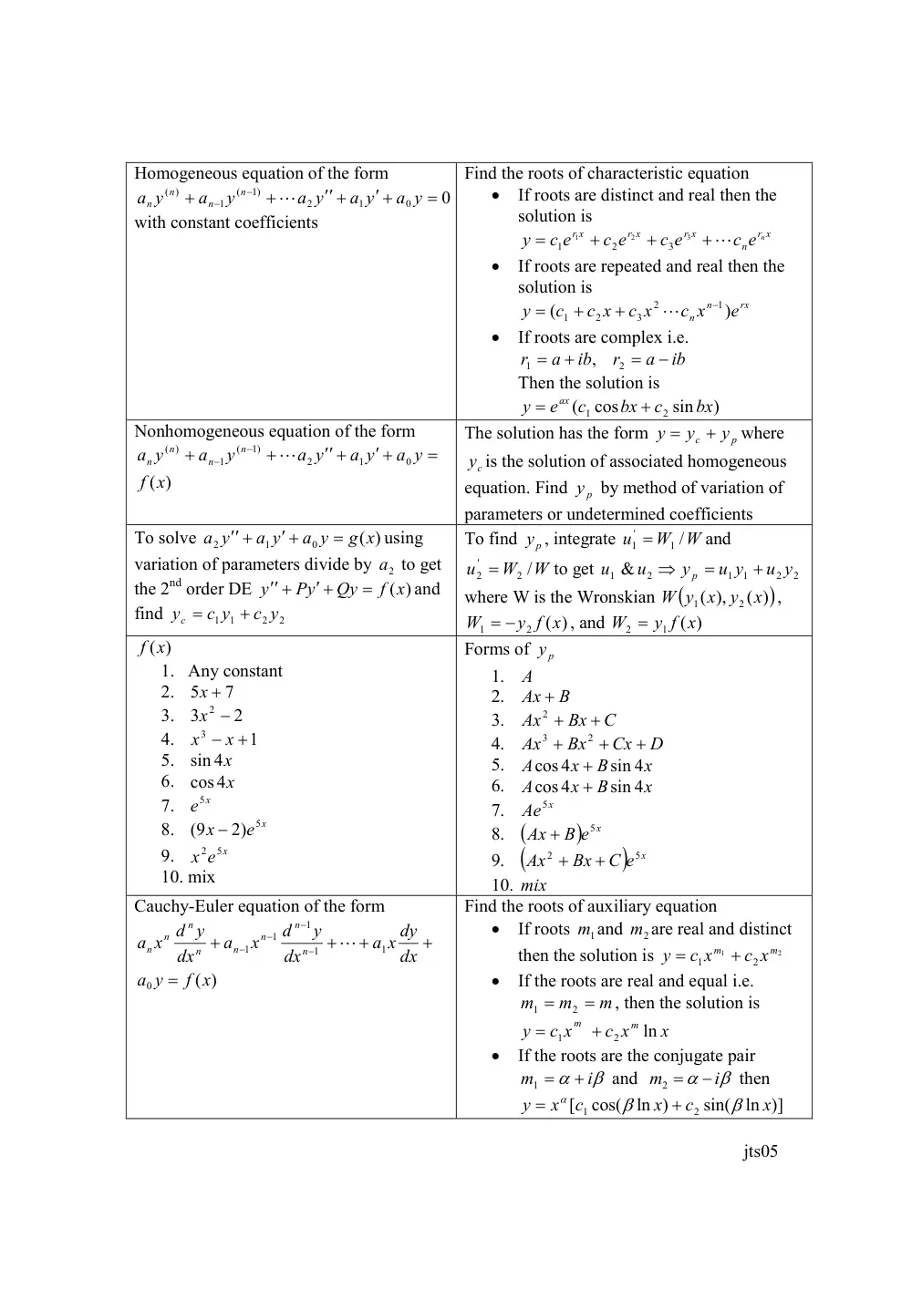If M M � y x − is a function of y alone, then multiply (E) by ∫ = − dy M M � y x e µ(y) Reduction of order can be used to find the general solution of a nonhomogeneous DE ( ) ( ) ( ) ' ) " ( 0 1 2 g x x y a x y a x y a = + + whenever a solution 1y is known ( ) ( ) ) ( 1 2 u x y x x y = can be obtained directly by: dx x y e y x y P x dx ∫ ∫ = − ( ) ) ( 2 1 ) ( 1 2 jts05 Homogeneous equation of the form 0 0 1 2 1) ( 1 ( ) = ′ + ′′ + + + − − a y a y a y y a y a n n n n L with constant coefficients Find the roots of characteristic equation • If roots are distinct and real then the solution is r x n r x r x r x c e n c e c e c e y +L + + = 3 2 1 3 2 1 • If roots are repeated and real then the solution is rx n n e c x c x c x c y ) ( 1 2 3 2 1 − + + = L • If roots are complex i.e. ib a r ib a r − = + = 2 1 , Then the solution is ) sin cos ( 2 1 bx c bx c e y ax + = Nonhomogeneous equation of the form ) ( 0 1 2 1) ( 1 ) ( x f a y a y a y y a y a n n n n = ′ + ′′ + + + − − L The solution has the form p c y y y + = where cy is the solution of associated homogeneous equation. Find p y by method of variation of parameters or undetermined coefficients To solve ) ( 0 1 2 g x a y a y a y = ′ + ′′ + using variation of parameters divide by 2 a to get the 2nd order DE f (x) Qy Py y = ′ + ′′ + and find 2 2 1 1 c y c y yc + = To find p y , integrate W W u 1 / ' 1 = and W W u 2 / ' 2 = to get 1u & u2 2 2 1 1 u y u y y p + = ⇒ where W is the Wronskian ( )) ( ), ( 2 1 x y W y x , ) ( 2 1 y f x W = − , and ) ( 1 2 W = y f x f (x) 1. Any constant 2. 5 + 7 x 3. 2 3 x2 − 4. 1 3 x − x + 5. sin 4x 6. cos4x 7. x e5 8. e x x 2) 5 (9 − 9. x e x 2 5 10. mix Forms of p y 1. A 2. Ax + B 3. C Bx Ax + 2 + 4. D Cx Bx Ax + + + 2 3 5. x B x A sin 4 cos4 + 6. x B x A sin 4 cos4 + 7. x Ae5 8. ( ) B e x Ax 5 + 9. ( ) C e x Bx Ax 5 2 + + 10. mix Cauchy-Euler equation of the form ) ( 0 1 1 1 1 1 f x a y dx a x dy dx y d x a dx x d y a n n n n n n n n = + + + + − − − − L Find the roots of auxiliary equation • If roots 1 m and 2 m are real and distinct then the solution is 2 1 2 1 m m c x c x y + = • If the roots are real and equal i.e. 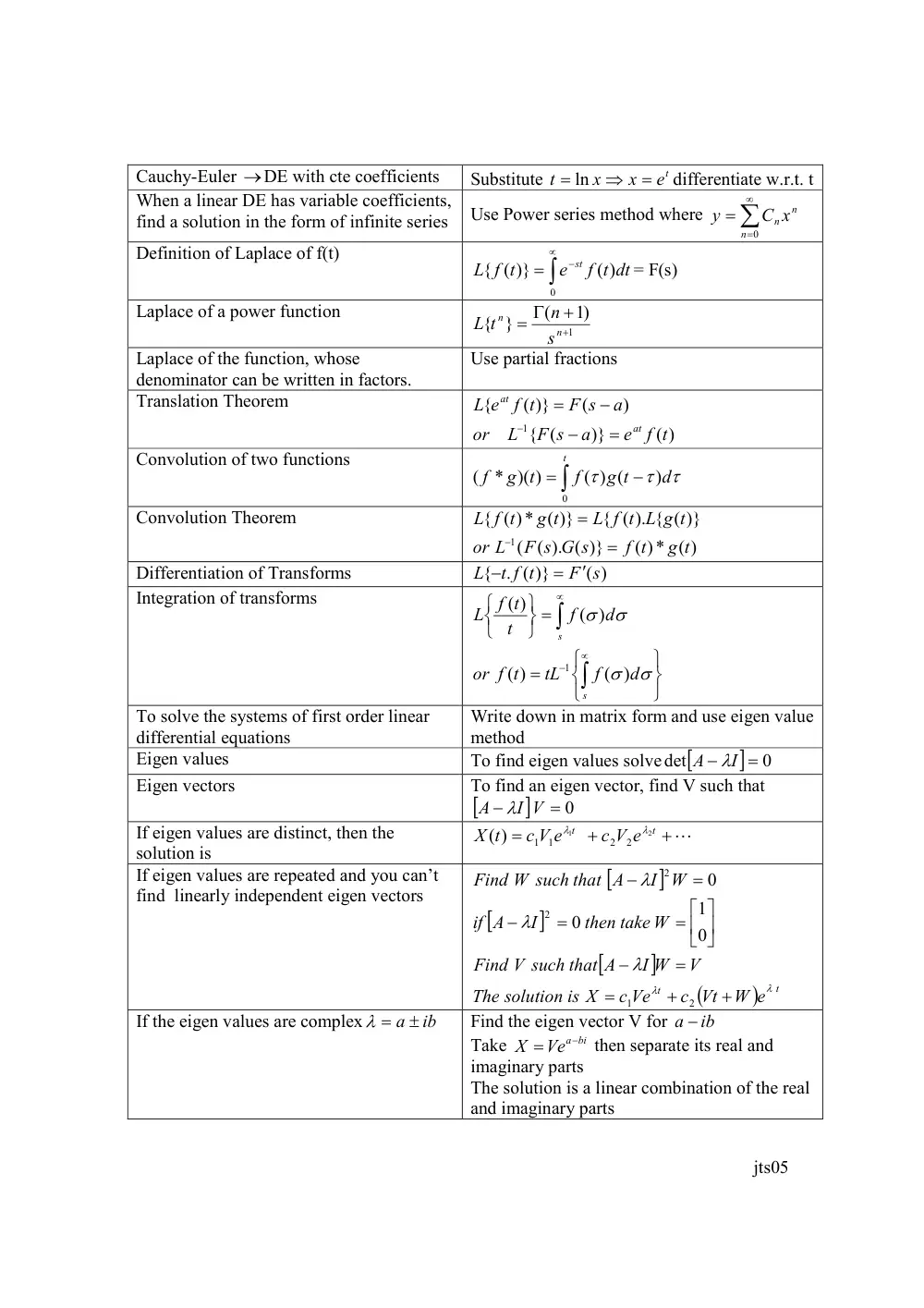m m m = = 2 1 , then the solution is x c x c x y m m ln 2 1 + = • If the roots are the conjugate pair β α i m + 1 = and β α i m − 2 = then ln )] sin( ln ) cos( [ 2 1 x c x c x y β β α + = jts05 Cauchy-Euler →DE with cte coefficients Substitute te x x t = ⇒ = ln differentiate w.r.t. t When a linear DE has variable coefficients, find a solution in the form of infinite series Use Power series method where n n Cnx y ∑ ∞ = = 0 Definition of Laplace of f(t) ∫ ∝ − = 0 ( ) { ( )} f t dt e f t L st = F(s) Laplace of a power function 1 )1 ( } { + + Γ = n n s n L t Laplace of the function, whose denominator can be written in factors. Use partial fractions Translation Theorem ( ) )} ( { ) ( ( )} { 1 f t e a F s L or a F s f t e L at at = − − = − Convolution of two functions ∫ − = t d g t f g t f 0 ) ( ) ( * )( ) ( τ τ τ Convolution Theorem ( )* ( ) ( ). ( )} ( { ( ). { ( )} ( )* ( )} { 1 g t f t F s G s L or L f t L g t g t f t L = = − Differentiation of Transforms ( ) . ( )} { F s t f t L ′ = − Integration of transforms       =  =  ∫ ∫ ∝ − ∝ s s d f tL f t or d f t f t L σ σ σ σ ( ) ) ( ( ) ) ( 1 To solve the systems of first order linear differential equations Write down in matrix form and use eigen value method Eigen values To find eigen values solve [ ] 0 det A − I = λ Eigen vectors To find an eigen vector, find V such that [ ] = 0 − I V A λ If eigen values are distinct, then the solution is +L + = t t c V e c V e t X 2 1 2 2 1 1 ( ) λ λ If eigen values are repeated and you can’t find linearly independent eigen vectors [ ] [ ] [ ] ( ) t t W e c Vt c Ve solution is X The V I W V such that A Find then take W I A if I W W such that A Find λ λ λ λ λ + + = = −    =  = − = − 2 1 2 2 0 1 0 0 If the eigen values are complex λ = a ± ib Find the eigen vector V for a − ib Take Vea bi X − = then separate its real and imaginary parts The solution is a linear combination of the real and imaginary parts