STAT 230 Chapter 2, Spring 2020

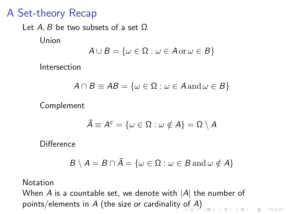
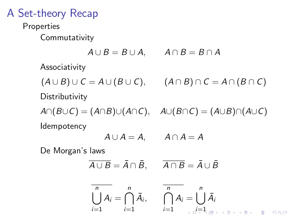
Chapter 2- 2020 Summer A Set-theory Recap Let A, B be two subsets of a set Ω Union A ∪ B = {ω ∈ Ω : ω ∈ A or ω ∈ B} Intersection A ∩ B ≡ AB = {ω ∈ Ω : ω ∈ A and ω ∈ B} Complement ¯A ≡ Ac = {ω ∈ Ω : ω /∈ A} = Ω \ A Difference B \ A = B ∩ ¯A = {ω ∈ Ω : ω ∈ B and ω /∈ A} Notation When A is a countable set, we denote with |A| the number of points/elements in A (the size or cardinality of A) A Set-theory Recap Properties Commutativity A ∪ B = B ∪ A, A ∩ B = B ∩ A Associativity (A ∪ B) ∪ C = A ∪ (B ∪ C), (A ∩ B) ∩ C = A ∩ (B ∩ C) Distributivity A∩(B∪C) = (A∩B)∪(A∩C), A∪(B∩C) = (A∪B)∩(A∪C) Idempotency A ∪ A = A, A ∩ A = A De Morgan’s laws A ∪ B = ¯A ∩ ¯B, A ∩ B = ¯A ∪ ¯B n� i=1 Ai = n� i=1 ¯Ai, n� i=1 Ai = n� i=1 ¯Ai A Set-theory Recap. Poincar´e Identities Inclusion-Exclusion Principle (Poincar´e Identity) Let Ai ⊂ Ω, i = 1, . . . , n | n� i=1 Ai| = |A1 ∪ A2 ∪ . . . ∪ An| = n � i=1 |Ai| − � 1≤i<j≤n |Ai ∩ Aj| + � 1≤i<j<k≤n |Ai ∩ Aj ∩ Ak| − . . . + (−1)n−1|A1 ∩ A2 ∩ . . . An| For example, for n = 3 |A∪B ∪C| = |A|+|B|+|C|−|A∩B|−|A∩C|−|B ∩C|+|A∩B ∩C| A Set-theory Recap. Poincar´e Identities Using the De Morgan’s law, it then follows | n� i=1 ¯Ai| = |Ω \ n� i=1 Ai| = |Ω| − | n� i=1 Ai| since Ω ⊇ n� i=1 Ai = |Ω| − n � i=1 |Ai| + � 1≤i<j≤n |Ai ∩ Aj| − � 1≤i<j<k≤n |Ai ∩ Aj ∩ Ak| + . . . + (−1)n−1|A1 ∩ A2 ∩ . . . An| An Example In a group of 21 (Arabic-speaking) Lebanese, 16 speak French, 13 English, 4 Armenian, 9 English and French, 2 French and Armenian, 3 English and Armenian and 1 English, French and Armenian. How many speak only Arabic? An Example In a group of 21 (Arabic-speaking) Lebanese, 16 speak French, 13 English, 4 Armenian, 9 English and French, 2 French and Armenian, 3 English and Armenian and 1 English, French and Armenian. How many speak only Arabic? Let A be the set of Armenophones, E the set of Anglophones, F the set of Francophones The set of those who speak only Arabic is An Example In a group of 21 (Arabic-speaking) Lebanese, 16 speak French, 13 English, 4 Armenian, 9 English and French, 2 French and Armenian, 3 English and Armenian and 1 English, French and Armenian. How many speak only Arabic? Let A be the set of Armenophones, E the set of Anglophones, F the set of Francophones The set of those who speak only Arabic is ¯A ∩ ¯E ∩ ¯F = A ∪ E ∪ F = Ω \ (A ∪ E ∪ F) | ¯A ∩ ¯E ∩ ¯F| = |Ω| − |A ∪ E ∪ F| = |Ω| − (|A| + |E| + |F|) + |A ∩ E| + |A ∩ F| + |E ∩ F| −|A ∩ E ∩ F| = 21 − (4 + 13 + 16) + 3 + 2 + 9 − 1 = 1 Sample Space and Events The sample space Ω (or S) associated with an experiment is the set of all possible outcomes of such an experiment Ω = {ω1, . . . , ωn} A subset E of Ω, E ⊂ Ω, is called an event Informally, an event is a statement on the outcomes of a random experiment We also assume that Ω is an event (the certain or universal event) if E is an event, so is its complement ¯E Hence, the empty set ∅ is an event (the impossible, or vacuous, event) the union of events is an event Sample Space and Events When E is just one outcome we say it is a simple event or a state (e.g. E = {ω3}) When E is more than one, we say it is a composite event or, simply, event (e.g. E = {ω2, ω21}) Sample Space Describe the sample spaces for the following experiments ▶ roll a regular die Sample Space Describe the sample spaces for the following experiments ▶ roll a regular die {1, 2, 3, 4, 5, 6} ▶ toss n coins (n = 4) Probability in a Simulation Roll a die, what is the probability of A =”3 appears”? The pseudo-code for the simulation to get the probability P(A) Problem How many ways can we roll three dice? In how many ways can three dice appear when they are rolled? How many possible numbers we get by rolling 3 dice (the order counts)? Some problems ▶ How many ways are there for 2 persons to sit in 7 chairs that are in a row? 7 · 6 = (7)2 Sampling (the chairs) with ordering (it matters in a theater, say, where you sit) and without replacement (two people may not sit on the same chair) ▶ How many ways are there to make a 3-letter word (a string of 3 letters) using a 26-letter alphabet? 263 ▶ How many ways are there to form a 3-letter word if the letters must be different? Sample Space Describe the sample spaces for the following experiments ▶ roll a regular die {1, 2, 3, 4, 5, 6} ▶ toss n coins (n = 4) {HHHH, HHHT, HHTH, HHTT, HTHH, HTTH, HTHT, HTTT, TTTT, TTTH, TTHT, TTHH, THTT, THHT, THTH, THHH} ▶ cast a regular die and, if 6 comes up, toss a coin Sample Space Describe the sample spaces for the following experiments ▶ roll a regular die {1, 2, 3, 4, 5, 6} ▶ toss n coins (n = 4) {HHHH, HHHT, HHTH, HHTT, HTHH, HTTH, HTHT, HTTT, TTTT, TTTH, TTHT, TTHH, THTT, THHT, THTH, THHH} ▶ cast a regular die and, if 6 comes up, toss a coin 6H, 6T, 1, 2, 3, 4, 5 ▶ measure the time for the emission of radioactive particle from some atom Sample Space Describe the sample spaces for the following experiments ▶ roll a regular die {1, 2, 3, 4, 5, 6} ▶ toss n coins (n = 4) {HHHH, HHHT, HHTH, HHTT, HTHH, HTTH, HTHT, HTTT, TTTT, TTTH, TTHT, TTHH, THTT, THHT, THTH, THHH} ▶ cast a regular die and, if 6 comes up, toss a coin 6H, 6T, 1, 2, 3, 4, 5 ▶ measure the time for the emission of radioactive particle from some atom (0, ∞) (this is a non-discrete case) Events Describe the events 1) when rolling a die, an even number comes up 2) when tossing n coins, the first n − 1 outcomes are tails 3) measuring the time for the emission of radioactive particle from some atom, the emission occurs after 3 minutes Events Describe the events 1) when rolling a die, an even number comes up 2) when tossing n coins, the first n − 1 outcomes are tails 3) measuring the time for the emission of radioactive particle from some atom, the emission occurs after 3 minutes 1) E = {2, 4, 6} 2) E = { n−1 � �� � TTTTTT T, n−1 � �� � TTTTTT H} 3) E = (3, ∞) (using minutes as unit of time) Sample Space and Events Events are subsets of a set, the sample space Ω Logical statements on events ⇐⇒ operation with sets Both event A and event B occur (conjunction) ⇐⇒ A ∩ B at least one of A and B occurs (disjunction)/ either A or B or both occur ⇐⇒ A ∪ B the event A does not occur (negation) ⇐⇒ ¯A the event A occurs but the event B does not ⇐⇒ A \ B Some Terminology If A ∩ B = ∅, A and B are said to be disjoint or incompatible or mutually exclusive events (that A and B both occur is impossible: the occurrence of one prevents the occurrence of the other) If A ⊆ B, A is said to imply B (B occurs if A occurs) In fact ⊆ is the set-theoretic equivalent of ⇒ Probability The first two elements of a probabilistic model are the sample space and the notion of events. The third element is the assignment of a probability to the events and outcomes of a random experiment We need to formalize statements such as the probability that when we roll a die an even number comes up is 1/2 Probability as Measure of Relative Frequencies One interpretation views probability as a relative frequency (which can be justified a posteriori by the result known as the law of large numbers) Carry out repeatedly and independently the same experiment a large number of times N (roll the same die in the same conditions N times) record the number of times SN(E) the event E occurs (”an even number comes up”) assign to the event the probability P(E) = SN(E)/N, N large, (the empirical limiting relative frequency in the N repetitions) Probability as Measure of Relative Frequencies The frequency definition of probability is based on the assumption that identical and independent experiments can be carried out (which is not always the case) A priori there is no guarantee that the relative frequency should converge to a limit and if that is the case, it is not clear how large N should be for the approximation to be reliable However even if there may be difficulties involved in defining probability in a mathematical form using repetitive events, this notion of probability is the basis of simulations, so you should keep it in mind Probability in a Simulation Roll a die, what is the probability of A =”3 appears”? The pseudo-code for the simulation to get the probability P(A) counter_a=0 for i from 1 to N roll a die if(die shows 3) counter_a = counter_a+1 end if end for return counter_a/N Probability in a Simulation. Implementation ▶ Python import numpy as np np.random.seed(164) N=1000000 die= np.arange(6)+1 a=np.random.choice(die, N, replace=True) np.count_nonzero(a==3)/N ▶ R set.seed(1364) N=1000000 a=sample(1:6, replace=T, N) length(which(a==3))/N ▶ Matlab rng(6356) N=1000000; a = randsample(6, N, true); sum(a==3)/N Probability In general, the assignment of a probability to an event is rather subtle Sometimes there are some natural choices, for example based on the existence of symmetries in the random experiment at hand Sometimes the choice will be subjective (probability assignments may differ from individual to individual) Let us now consider a mathematical (axiomatic) definition of probability: probability as a function that satisfies some properties (a version of these properties are indeed verified by the relative frequency) Discrete Probability Space Let the sample space Ω be non-empty and countable for the rest of this chapter Third element necessary to complete the description of a probabilistic model is a function P : Set of Events −→ [0, 1] called probability that verifies the following two axioms A1) P(Ω) = 1 The certain event has probability 1 A2) σ-additivity (countable additivity) For every sequence (Ai)i∈N of disjoint/mutually exclusive events, Ai ∩ Aj = ∅, i ̸= j P � ∞ � i=1 Ai � = ∞ � i=1 P(Ai) (Ω, P) is called a discrete probability space, with Ω its sample space, and subsets of Ω the events Probability. Properties For a discrete probability space (Ω, P), the following statements hold true (all follow from A1 and A2) S1) The impossible event has probability zero P(∅) = 0 Proof. If Ai = ∅, i ∈ N, then �∞ i=1 Ai = ∅ P(∅) = P � ∞ � i=1 Ai � = ∞ � i=1 P(Ai) = ∞ � i=1 P(∅) which holds iff P(∅) = 0. Probability. Properties S2) Finite additivity Let Ai, i = 1, . . . , n, be a finite family of disjoint events, Ai ∩ Aj = ∅, i ̸= j P � n� i=1 Ai � = n � i=1 P(Ai) This follows from countable additivity, A2, setting Ak = ∅ for all k ≥ n. Thus it is a weaker notion than countable additivity. When Ω is finite, we can equally define the probability space using axioms A1 and A2 or A1 and S2 (finite additivity) Probability. Properties Other consequences of A1 and A2 (draw the corresponding Venn diagram if in doubt) S3) P( ¯A) = 1 − P(A) 1 = P(Ω) = P(A ∪ ¯A) = P(A) + P( ¯A) since A ∩ ¯A = ∅ S4) For any A, B ⊆ Ω P(B \ A) = P(B) − P(A ∩ B) Since B = (B \ A) ∪ (A ∩ B), with B \ A and (A ∩ B) disjoint, then P(B) = P(B \ A) + P(A ∩ B) hence the result Probability. Properties S5) For any or any A, B ⊆ Ω P(A ∪ B) = P(A) + P(B) − P(A ∩ B) Since A ∪ B = A ∪ (B \ A), and A and B \ A are disjoint, P(A ∪ B) = P(A) + P(B \ A) = P(A) + P(B) − P(A ∩ B) using S4 Inclusion-Exclusion Formulae (Poincar´e’s Identities) (Ω, P) a discrete probability space. For any n ≥ 1 and for any choice of sets (events) A1, . . . An ⊆ Ω P(A1 ∪ . . . ∪ An) = n � k=1 (−)k−1 � 1≤i1<...<ik≤n P(Ai1 ∩ . . . ∩ Aik) P(A1 ∩ . . . ∩ An) = n � k=1 (−)k−1 � 1≤i1<...<ik≤n P(Ai1 ∪ . . . ∪ Aik) They can be proven by induction They are actually valid on any probability space (finite, countable or uncountable) Example For example for n = 4, calling the events A1 = A, A2 = B, A3 = C, A4 = D P(A ∪ B ∪ C ∪ D) = P(A) + P(B) + P(C) + P(D) −P(A ∩ B) − P(A ∩ C) − P(A ∩ D) −P(B ∩ C) − P(B ∩ D) − P(C ∩ D) +P(A ∩ B ∩ C) + P(A ∩ B ∩ D) +P(A ∩ C ∩ D) + P(B ∩ C ∩ D) −P(A ∩ B ∩ C ∩ D) Alternating sum of the probabilities of each event (4 terms), each possible pair of events (6), each possible triple of events (4), each possible quadruple (1) When to use the Poincar´e formula Very often if one has to compute the probability that at least one event occurs or the probability that no event occurs, the Poincar´e formula is most useful Indeed, let Ai be i = 1, . . . , n n events P(A1 ∪ . . . ∪ An) is the probability that at least one of the n events occurs P( ¯A1 ∩ . . . ∩ ¯An) is the probability that none occurs By the Poincar´e formulae, these probabilities can be written in terms of probability involving fewer events, which are often easier to compute Probability of events and outcomes (Ω, P) discrete probability space, A = {ωi1, . . . , ωik} a compound event, then its probability is P(A) = k � j=1 P(ωij) with the restriction 1 = P(Ω) = � ω∈Ω P(ω) Example Ω = {ω1, ω2, ω3, ω4} P(ωi) = p, ∀i A1 = {ω1, ω2}, A2 = {ω1, ω3}, A3 = {ω1, ω4} Find P(Ai), P(Ai ∩ Aj), P(A1 ∩ A2 ∩ A3), P(Ai ∪ Aj) etc. Probability of events and outcomes (Ω, P) discrete probability space, A = {ωi1, . . . , ωik} a compound event, then its probability is P(A) = k � j=1 P(ωij) with the restriction 1 = P(Ω) = � ω∈Ω P(ω) Example Ω = {ω1, ω2, ω3, ω4} P(ωi) = p, ∀i A1 = {ω1, ω2}, A2 = {ω1, ω3}, A3 = {ω1, ω4} Find P(Ai), P(Ai ∩ Aj), P(A1 ∩ A2 ∩ A3), P(Ai ∪ Aj) etc. P(ωi) = 1/4, P(Ai) = 2/4, P(Ai ∩ Aj) = 1/4 = P(A1 ∩ A2 ∩ A3) P(Ai ∪ Aj) = 3/4, P(A1 ∪ A2 ∪ A3) = P(Ω) = 1 Uniform Probability Space A discrete probability space (Ω, P) which is finite (that is, Ω is finite) and such that the outcomes ωi ∈ Ω are equiprobable is called a uniform probability space. In this case, then P(ωi) = 1/|Ω| The previous page example is such a space More generally for any event E (a subset of Ω) P(E) = |E| |Ω| The probability of an event is the ratio of the number of cases that are favorable to it, to the number of possible cases, when there is nothing to make us believe that one case should occur rather than any other [Laplace] Thus the problem of computing a probability of an event becomes the problem of counting the number of its elements Equiprobability It is necessary that all points in the sample space be equiprobable for computing probability via simple counting P(E) = |E|/|Ω| Suppose we want to compute the probability of getting a three by summing the numbers that turn up on tossing two dice E = ”the sum of two throws is 3” Since the sum is symmetric, we can think of using the following sample space, where [i, j] is the unordered couple, with i the number for one of the dice and j for the other ˜Ω =         [1, 1] [1, 2] [1, 3] [1, 4] [1, 5] [1, 6] [2, 2] [2, 3] [2, 4] [2, 5] [2, 6] [3, 3] [3, 4] [3, 5] [3, 6] [4, 4] [4, 5] [4, 6] [5, 5] [5, 6] [6, 6]         Equiprobability While there may be nothing wrong in using ˜Ω, it should be noticed however its simple events are not equally probable For example, p([1, 1]) = 1/36 p([1, 2]) = p((1, 2) ∪ (2, 1)) = p((1, 2)) + p((2, 1)) = 2/36, [i, j] unordered couple, (i, j) ordered couple [i, j] one die shows the i-th face the other the j-th face (i, j) the first die shows i the second j, if we throw them one after the other or, if you toss them at the same time, just color the dice differently: the red die shows i, the blue die j [i, j] = {(i, j), (j, i)} Thus we may not compute the probability by simple counting the number of the points in the space that are favorable to the event (one point [1, 2]) and divide by the size of the space 21 We would get 1/21, instead of the correct probability which is 2/36 Equiprobability Instead we can use the following equiprobable sample space Ω =         (1, 1) (1, 2) (1, 3) (1, 4) (1, 5) (1, 6) (2, 1) (2, 2) (2, 3) (2, 4) (2, 5) (2, 6) (3, 1) (3, 2) (3, 3) (3, 4) (3, 5) (3, 6) (4, 1) (4, 2) (4, 3) (4, 4) (4, 5) (4, 6) (5, 1) (5, 2) (5, 3) (5, 4) (5, 5) (5, 6) (6, 1) (6, 2) (6, 3) (6, 4) (6, 5) (6, 6)         whose |Ω| = 36 outcomes are all equiprobable P((i, j)) = 1/36, thus |E = {i + j = 3}| = 2, P(E) = |E|/|Ω| = 2/36 More generally (exercise) the probability of rolling a sum of k, with two dice is P({i + j = k}) = 6 − |7 − k| 36 , k = 2, . . . , 12 Combinatorics. Multiplication Rule First rule of counting. Multiplication Rule If an object is formed by making a succession of choices such that there are n1 possibilities for the first choice, n2 possibilities for the second (after the first choice is made) etc. then the total number of objects that can be made by making a set of choices is |E| = n1 · n2 · · · For the rule to apply, the number of available possibilities of each choice must be the same irrespective of which choice was made previously (ni for the i-th choice, which may be different from nj). However the set of available possibilities may differ and depend on the choice made at the previous stages Book Problem 31 Beethoven wrote 9 symphonies, 5 piano concertos, and 32 piano sonatas. a) How many ways are there to play first a Beethoven symphony and then a Beethoven piano concerto? Book Problem 31 Beethoven wrote 9 symphonies, 5 piano concertos, and 32 piano sonatas. a) How many ways are there to play first a Beethoven symphony and then a Beethoven piano concerto? 9 · 5 = 45 You may find it helpful to draw a tree b) The manager of a radio station decides that on each successive evening (7 days per week), a Beethoven symphony will be played followed by a Beethoven piano concerto followed by a Beethoven piano sonata. For how many years could this policy be continued before exactly the same program would have to be repeated? Book Problem 31 Beethoven wrote 9 symphonies, 5 piano concertos, and 32 piano sonatas. a) How many ways are there to play first a Beethoven symphony and then a Beethoven piano concerto? 9 · 5 = 45 You may find it helpful to draw a tree b) The manager of a radio station decides that on each successive evening (7 days per week), a Beethoven symphony will be played followed by a Beethoven piano concerto followed by a Beethoven piano sonata. For how many years could this policy be continued before exactly the same program would have to be repeated? 9 · 5 · 32 = 1440 days ≈ 4 years Problem How many ways can we roll three dice? In how many ways can three dice appear when they are rolled? How many possible numbers we get by rolling 3 dice (the order counts)? We have a succession of three choices (one per die) and each die represents a multiple choice of six possibilities ni = 6, thus there are 6 · 6 · 6 = 216 possible rolls This is obvious if you think of tossing the dice one after the other rather than simultaneously (although it does not matter) The set of choices at each throw of the dice in this case does not change based on what happens at the previous stage (it is always one of the numbers {1, 2, 3, 4, 5, 6} (and thus the number does not change which is only thing that matters for the multiplicative rule) Problem In how many ways can two dice show different faces? Problem In how many ways can two dice show different faces? 6 · 5 In this case there are 6 available possibilities for the first choice. Five different possibilities for the second die. Which five depends on the first choice (e.g. if 3 shows up on the first roll, the set of available possibilities is {1, 2, 4, 5, 6}, if 2 shows up, such set is {1, 3, 4, 5, 6}), but there are always 5 possibilities for the second die, so the first rule of counting as formulated above still applies Problem How many different calendars are possible for a year? Problem How many different calendars are possible for a year? 7 · 2 = 14 Each year starts on one of the seven days (Sunday, Monday, ..., Saturday). Each year is either a leap year (i.e., it includes February 29) or not Standard Ways of Counting and Basic Probabilistic Models We are going to see now two standard ways of counting which can be used in the majority of combinatorial problems ▶ Sampling Methods ▶ Allocation Methods Basic Probabilistic Models. Sampling Model Consider a population of n individuals (people, cards, numbered balls), i.e. an aggregate of n distinguishable elements without regard to their order (think of an urn containing nF numbered balls) Choose an individual from the population (a sample of size 1) (that is, draw one ball from the urn) How many ways can we do this? Basic Probabilistic Models. Sampling Model Consider a population of n individuals (people, cards, numbered balls), i.e. an aggregate of n distinguishable elements without regard to their order (think of an urn containing nF numbered balls) Choose an individual from the population (a sample of size 1) (that is, draw one ball from the urn) How many ways can we do this? The answer is n Choose k individuals successively, one at a time How many ways can we do this? Basic Probabilistic Models. Sampling Model Consider a population of n individuals (people, cards, numbered balls), i.e. an aggregate of n distinguishable elements without regard to their order (think of an urn containing nF numbered balls) Choose an individual from the population (a sample of size 1) (that is, draw one ball from the urn) How many ways can we do this? The answer is n Choose k individuals successively, one at a time How many ways can we do this? It depends Basic Probabilistic Models. Sampling Model It depends on whether or not a chosen individual is returned to the population before another is chosen (that is, on whether or not we put the ball we have drawn back into the urn) It also depends on whether the sample of size k is ordered or not (namely, ordering means that the same individuals chosen in a different order are considered to be a different sample- drawing 1 before 2 is considered different from drawing 2 before 1) The two kinds of sampling models are called sampling with replacement we put the drawn ball back into the urn or we replace the ball we have drawn in the urn sampling without replacement we do not replace the drawn balls In addition we need to consider the sample to be ordered or un-ordered Basic Probabilistic Models Thus we will consider the following 2 · 2 = 4 cases ▶ Sampling with replacement and with ordering ▶ Sampling without replacement and with ordering ▶ Sampling without replacement and without ordering ▶ Sampling with replacement and without ordering Sampling with replacement and with ordering I. Sampling with replacement and with ordering The first individual is from a population with n individuals n1 = n We return the individual to the population, thus the set (and hence the number) of possibilities for the choice of a second individual is the same as for the first n2 = n Thus repeating the argument, using the multiplication rule (first rule), we find that there are n1 · · · nk = n · · · n = nk ways to draw an (ordered) sample of size k from a population of n individuals Sampling with replacement and with ordering nk counts the number of different ordered k-tuple from a population of size n Ordering means, e.g., that (1, 2, 1, 3) is considered different from (1, 2, 3, 1), (2, 1, 3, 1), etc. Put it differently, the sample space Ω is the set of ordered k-tuples Ω = {(a1, a2, . . . , ak), ai = 1, ..., n} Let us write down explicitly the number of ordered samples of size k = 2 that can be obtained from n = 3 objects, if an object may appear more than once (”sampling with replacement”) Sampling with replacement and with ordering nk counts the number of different ordered k-tuple from a population of size n Ordering means, e.g., that (1, 2, 1, 3) is considered different from (1, 2, 3, 1), (2, 1, 3, 1), etc. Put it differently, the sample space Ω is the set of ordered k-tuples Ω = {(a1, a2, . . . , ak), ai = 1, ..., n} Let us write down explicitly the number of ordered samples of size k = 2 that can be obtained from n = 3 objects, if an object may appear more than once (”sampling with replacement”) (1, 1), (1, 2), (1, 3) (2, 1), (2, 2), (2, 3) (3, 1), (3, 2), (3, 3)