STAT 230 Lecture Chapter 3, Fall 2011

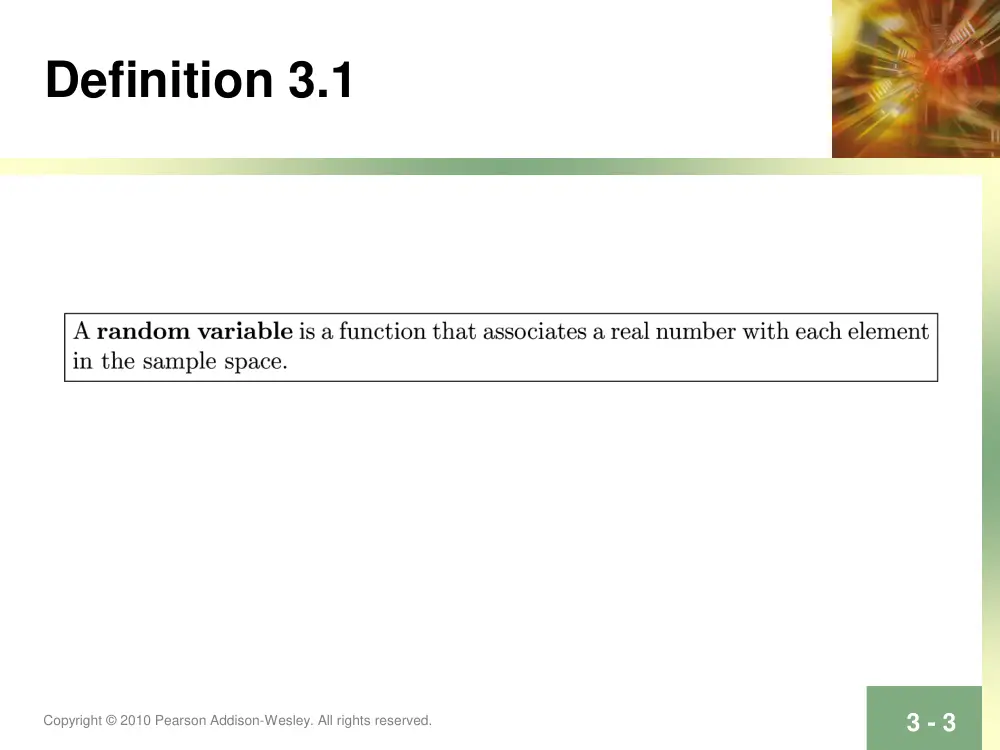
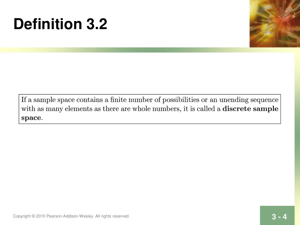
Copyright © 2010 Pearson Addison-Wesley. All rights reserved. Chapter 3 Random Variables and Probability Distributions Copyright © 2010 Pearson Addison-Wesley. All rights reserved. Section 3.1 Concept of a Random Variable Copyright © 2010 Pearson Addison-Wesley. All rights reserved. 3 - 3 Definition 3.1 Copyright © 2010 Pearson Addison-Wesley. All rights reserved. 3 - 4 Definition 3.2 Copyright © 2010 Pearson Addison-Wesley. All rights reserved. 3 - 5 Definition 3.3 Copyright © 2010 Pearson Addison-Wesley. All rights reserved. Section 3.2 Discrete Probability Distribution Copyright © 2010 Pearson Addison-Wesley. All rights reserved. 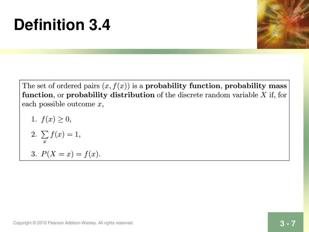3 - 7 Definition 3.4 Copyright © 2010 Pearson Addison-Wesley. All rights reserved. 3 - 8 Definition 3.5 Copyright © 2010 Pearson Addison-Wesley. All rights reserved. 3 - 9 Figure 3.1 Probability mass function plot Copyright © 2010 Pearson Addison-Wesley. All rights reserved. 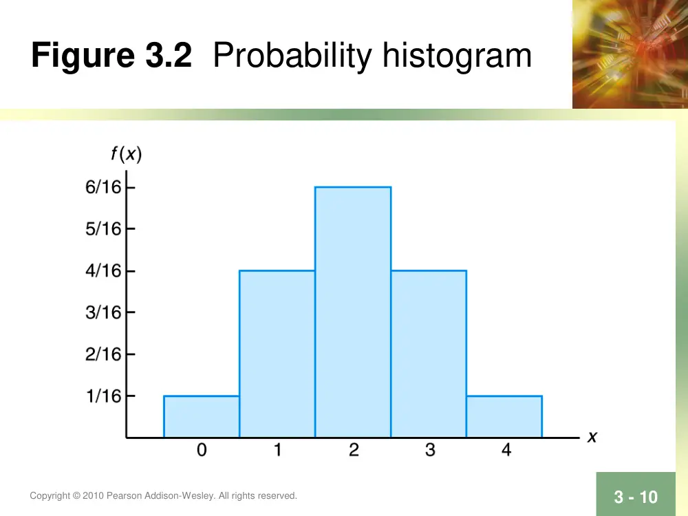3 - 10 Figure 3.2 Probability histogram Copyright © 2010 Pearson Addison-Wesley. All rights reserved. 3 - 11 Figure 3.3 Discrete cumulative distribution function Copyright © 2010 Pearson Addison-Wesley. All rights reserved. Section 3.3 Continuous Probability Distributions Copyright © 2010 Pearson Addison-Wesley. All rights reserved. 3 - 13 Figure 3.4 Typical density functions Copyright © 2010 Pearson Addison-Wesley. All rights reserved. 3 - 14 Figure 3.5 P(a < X < b) Copyright © 2010 Pearson Addison-Wesley. All rights reserved. 3 - 15 Definition 3.6 Copyright © 2010 Pearson Addison-Wesley. All rights reserved. 3 - 16 Definition 3.7 Copyright © 2010 Pearson Addison-Wesley. All rights reserved. 3 - 17 Figure 3.6 Continuous cumulative distribution function Copyright © 2010 Pearson Addison-Wesley. All rights reserved. Section 3.4 Joint Probability Distributions Section Abstract • We generalize the concept of distribution of a single random variable to the case of two r.v.’s where we speak of their joint distribution. We do so by introducing: 1. The joint p.f. of two discrete r.v.’s 2. The joint p.d.f. of two continuous r.v.’s 3. The joint d.f. for any two r.v.’s Copyright © 2010 Pearson Addison-Wesley. All rights reserved. 3 - 20 Definition 3.8 Copyright © 2010 Pearson Addison-Wesley. All rights reserved. 3 - 21 Table 3.1 Joint Probability Distribution for Example 3.14 Discrete Joint Distributions • Definition by example: A subcommittee of five members is to be formed randomly from among a committee of 10 democrats, 8 republicans and 2 independent members. • Let X and Y be the numbers of democrats and republicans chosen to serve on the committee, respectively. Their joint p.f. is: P(x,y):=P(X = x,Y = y) = C10,xC8,yC2,5-x-y / C20,5 X = 0,1,…,5; y = 0,1,…,5; x+y ≤ 5 and x+y ≥ 3 Copyright © 2010 Pearson Addison-Wesley. All rights reserved. 3 - 23 Definition 3.9 A Typical Shape Copyright © 2010 Pearson Addison-Wesley. All rights reserved. 3 - 25 Definition 3.10 Copyright © 2010 Pearson Addison-Wesley. All rights reserved. 3 - 26 Table 3.1 Joint Probability Distribution for Example 3.14 Copyright © 2010 Pearson Addison-Wesley. All rights reserved. 3 - 27 Definition 3.11 Copyright © 2010 Pearson Addison-Wesley. All rights reserved. 3 - 28 Definition 3.12 (Independence of random Variables) Copyright © 2010 Pearson Addison-Wesley. All rights reserved. 3 - 29 Definition 3.13 Example • Roll a fair die once and let X be the number of dots. • Toss a fair coin X times and let Y be the number of heads. Find the joint p.m.f. of X and Y. Copyright © 2010 Pearson Addison-Wesley. All rights reserved. 3 - 30 Example: Table of p(x,y) x y 0 1 2 3 4 5 6 pX(x) 1 1/12 1/12 0 0 0 0 0 1/6 2 1/24 2/24 1/24 0 0 0 0 1/6 3 1/48 3/48 3/48 1/48 0 0 0 1/6 4 1/96 4/96 6/96 4/96 1/96 0 0 1/6 5 1/192 5/192 10/192 10/192 5/192 1/192 0 1/6 6 1/384 6/384 15/384 20/384 15/384 6/384 1/384 1/6 pY(y) 63/384 120/384 99/384 64/384 29/384 8/384 1/384 1 Marginal distribution of X x y 0 1 2 3 4 5 6 pX(x) 1 1/12 1/12 0 0 0 0 0 1/6 2 1/24 2/24 1/24 0 0 0 0 1/6 3 1/48 3/48 3/48 1/48 0 0 0 1/6 4 1/96 4/96 6/96 4/96 1/96 0 0 1/6 5 1/192 5/192 10/192 10/192 5/192 1/192 0 1/6 6 1/384 6/384 15/384 20/384 15/384 6/384 1/384 1/6 pY(y) 63/384 120/384 99/384 64/384 29/384 8/384 1/384 1 Marginal distribution of Y x y 0 1 2 3 4 5 6 pX(x) 1 1/12 1/12 0 0 0 0 0 1/6 2 1/24 2/24 1/24 0 0 0 0 1/6 3 1/48 3/48 3/48 1/48 0 0 0 1/6 4 1/96 4/96 6/96 4/96 1/96 0 0 1/6 5 1/192 5/192 10/192 10/192 5/192 1/192 0 1/6 6 1/384 6/384 15/384 20/384 15/384 6/384 1/384 1/6 pY(y) 63/384 120/384 99/384 64/384 29/384 8/384 1/384 1 Examples Find the constant c that renders the function f(x,y) into a joint p.d.f.: • f(x,y)= cxy2; 0 ≤ x ≤ 1; 0 ≤ y ≤ 1 AND zero elsewhere • f(x,y)= cxy2; 0 ≤ x ≤ y ≤ 1 AND zero elsewhere Find P(X>3/4) in each case. Will the Chicken Be Safe? • A farmer wants to build a triangular pen for his chickens. He sends his son out to cut the lumber and the boy, without taking any thought as to the ultimate purpose, makes two cuts at two points selected at random. What are the chances that the resulting three pieces can be used to form a triangular pen? Will the Chicken Be Safe? • Suppose that the length of the lumber is L • Let X and Y be the distances from the left to the two points where the cuts “occur” • Two cases: (1) X < Y and (2) Y < X Case1: pieces have lengths: X, Y-X, L-Y Case2: pieces have lengths: Y, X-Y, L-X. By symmetry, both cases have the same probability Will the Chicken Be Safe? Case 1: the three pieces form a triangle iff The length of any piece is less than the sum of the other two. We get the restrictions: X < Y X < (Y-X) + (L-Y) => X < L/2 (Y-X) < X + (L-Y) => (Y-X) < L/2 L-Y < X + (Y-X) => Y > L/2 Will the Chicken Be Safe? • So the conditions are X < Y; X < L/2; (Y-X) < L/2; Y > L/2. • Then integrate the joint pdf of X and Y in the domain determined by those conditions. Note: (X,Y) is a point taken uniformly from the square 0 < X < L, 0 < Y < L, Hence it has denisty f(x,y) =1/L2 in that square and zero elsewhere