COE 799 Project 2, Fall 2011

L E B A N E S E A M E R I C A N U N I V E R S I T Y Electrical and Computer Engineering Dept COE 799 Optical Networks Fall 2011 W. FAWAZ Project II Due Date: Thursday January 19 2012 Kindly note that the description presented below can also be found on page 236 of your textbook. Objective The objective of this simulation project is to calculate the blocking probability of dynamically arriving call requests for the establishment of lightpaths in a network of OXCs. Each OXC may have no converters, partial conversion, or full conversion. 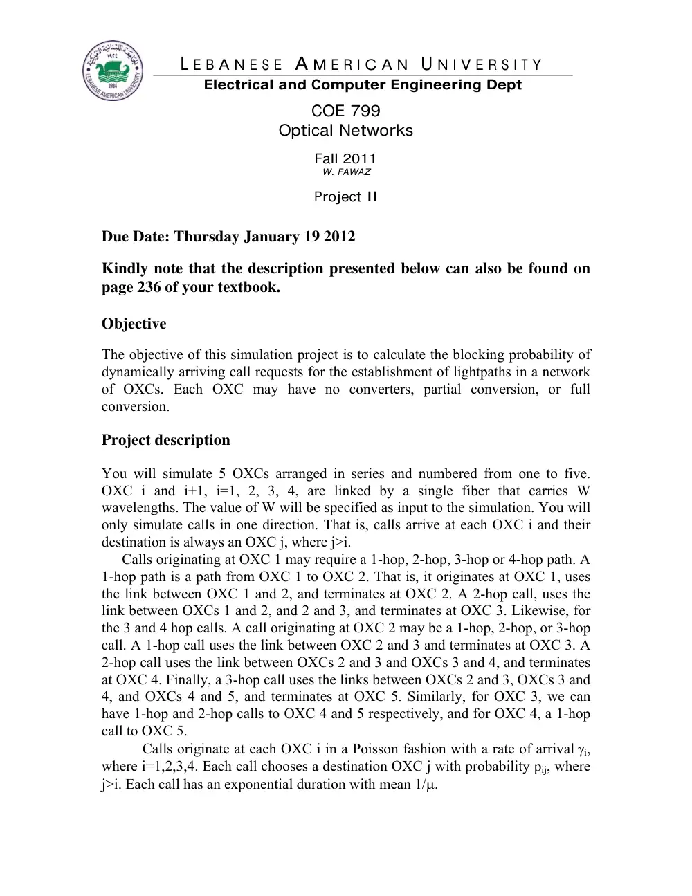Project description You will simulate 5 OXCs arranged in series and numbered from one to five. OXC i and i+1, i=1, 2, 3, 4, are linked by a single fiber that carries W wavelengths. The value of W will be specified as input to the simulation. You will only simulate calls in one direction. That is, calls arrive at each OXC i and their destination is always an OXC j, where j>i. Calls originating at OXC 1 may require a 1-hop, 2-hop, 3-hop or 4-hop path. A 1-hop path is a path from OXC 1 to OXC 2. That is, it originates at OXC 1, uses the link between OXC 1 and 2, and terminates at OXC 2. A 2-hop call, uses the link between OXCs 1 and 2, and 2 and 3, and terminates at OXC 3. Likewise, for the 3 and 4 hop calls. A call originating at OXC 2 may be a 1-hop, 2-hop, or 3-hop call. A 1-hop call uses the link between OXC 2 and 3 and terminates at OXC 3. A 2-hop call uses the link between OXCs 2 and 3 and OXCs 3 and 4, and terminates at OXC 4. Finally, a 3-hop call uses the links between OXCs 2 and 3, OXCs 3 and 4, and OXCs 4 and 5, and terminates at OXC 5. Similarly, for OXC 3, we can have 1-hop and 2-hop calls to OXC 4 and 5 respectively, and for OXC 4, a 1-hop call to OXC 5. Calls originate at each OXC i in a Poisson fashion with a rate of arrival γi, where i=1,2,3,4. Each call chooses a destination OXC j with probability pij, where j>i. Each call has an exponential duration with mean 1/µ. 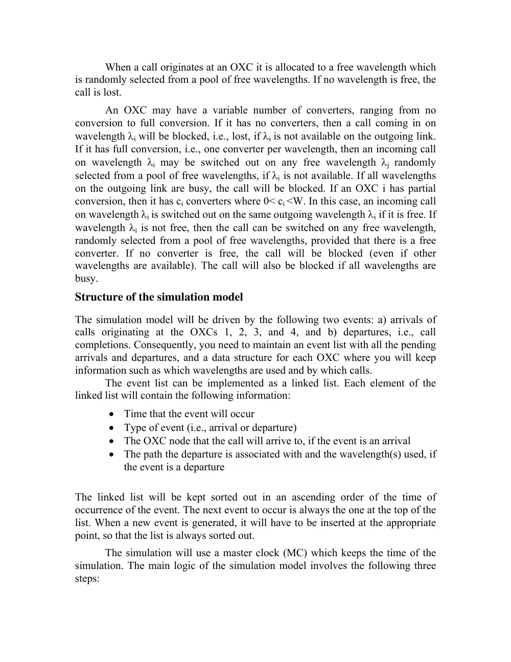When a call originates at an OXC it is allocated to a free wavelength which is randomly selected from a pool of free wavelengths. If no wavelength is free, the call is lost. An OXC may have a variable number of converters, ranging from no conversion to full conversion. If it has no converters, then a call coming in on wavelength λi will be blocked, i.e., lost, if λi is not available on the outgoing link. If it has full conversion, i.e., one converter per wavelength, then an incoming call on wavelength λi may be switched out on any free wavelength λj randomly selected from a pool of free wavelengths, if λi is not available. If all wavelengths on the outgoing link are busy, the call will be blocked. If an OXC i has partial conversion, then it has ci converters where 0< ci <W. In this case, an incoming call on wavelength λi is switched out on the same outgoing wavelength λi if it is free. If wavelength λi is not free, then the call can be switched on any free wavelength, randomly selected from a pool of free wavelengths, provided that there is a free converter. If no converter is free, the call will be blocked (even if other wavelengths are available). The call will also be blocked if all wavelengths are busy. Structure of the simulation model The simulation model will be driven by the following two events: a) arrivals of calls originating at the OXCs 1, 2, 3, and 4, and b) departures, i.e., call completions. Consequently, you need to maintain an event list with all the pending arrivals and departures, and a data structure for each OXC where you will keep information such as which wavelengths are used and by which calls. The event list can be implemented as a linked list. Each element of the linked list will contain the following information: • Time that the event will occur • Type of event (i.e., arrival or departure) • The OXC node that the call will arrive to, if the event is an arrival • The path the departure is associated with and the wavelength(s) used, if the event is a departure The linked list will be kept sorted out in an ascending order of the time of occurrence of the event. The next event to occur is always the one at the top of the list. When a new event is generated, it will have to be inserted at the appropriate point, so that the list is always sorted out. The simulation will use a master clock (MC) which keeps the time of the simulation. 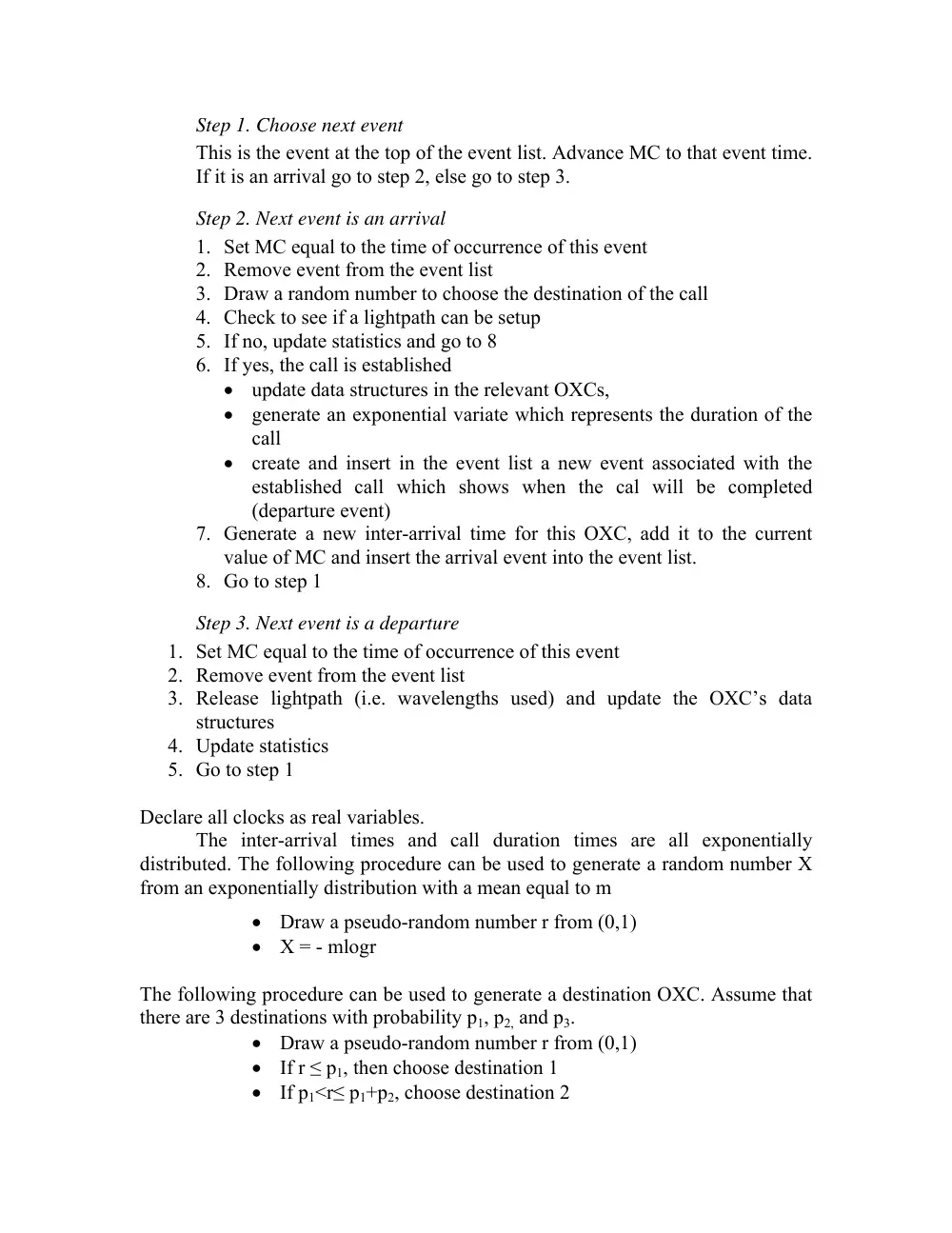The main logic of the simulation model involves the following three steps: Step 1. Choose next event This is the event at the top of the event list. Advance MC to that event time. If it is an arrival go to step 2, else go to step 3. Step 2. Next event is an arrival 1. Set MC equal to the time of occurrence of this event 2. Remove event from the event list 3. Draw a random number to choose the destination of the call 4. Check to see if a lightpath can be setup 5. If no, update statistics and go to 8 6. If yes, the call is established • update data structures in the relevant OXCs, • generate an exponential variate which represents the duration of the call • create and insert in the event list a new event associated with the established call which shows when the cal will be completed (departure event) 7. Generate a new inter-arrival time for this OXC, add it to the current value of MC and insert the arrival event into the event list. 8. Go to step 1 Step 3. Next event is a departure 1. Set MC equal to the time of occurrence of this event 2. Remove event from the event list 3. Release lightpath (i.e. wavelengths used) and update the OXC’s data structures 4. Update statistics 5. Go to step 1 Declare all clocks as real variables. The inter-arrival times and call duration times are all exponentially distributed. The following procedure can be used to generate a random number X from an exponentially distribution with a mean equal to m • Draw a pseudo-random number r from (0,1) • X = - mlogr The following procedure can be used to generate a destination OXC. Assume that there are 3 destinations with probability p1, p2, and p3. • Draw a pseudo-random number r from (0,1) • If r ≤ p1, then choose destination 1 • If p1<r≤ p1+p2, choose destination 2 • Else, if r> p1+p2 , choose destination 3. Remember to draw a new pseudo-random number every time you need one!! The simulation will run until a predefined number of departures, given as input to the simulation, occur. Simulation inputs The inputs are: W, number of converters ci for each OXC i, where i=1,2,3,4,5, the arrival rates γi, where i=1,2,3,4, destination probabilities pij, where i=1,2,3,4,5, j=2,3,4,5, and i<j, the mean call duration 1/µ; and the simulation run (i.e., the number of simulated departures). Simulation outputs Calculate the total call blocking probability over all paths and also the call blocking probabilities for each path (i,j), where i=1,2,3,4, j=2,3,4,5 and i<j. Present your results for the path call blocking probability in a graph where each point on the x-axis represents a path. To calculate the output statistics, run your simulation for 100 departures (warm-up period), initialize all your statistic counters and then run it for the total number of departures specified as input to the simulation. If your curves are not smooth, increase the simulation run. Debugging Run your simulation for several departures, and then print out the content of all the variables in your simulation, each time an arrival or a departure occurs. Go over the print out by hand and verify that the logic of your program is correct. That is, it advances correctly from event to event, and for each event the data structures are correctly maintained. This is a boring exercise, but it is the only way that you can make sure that your simulation works correctly! 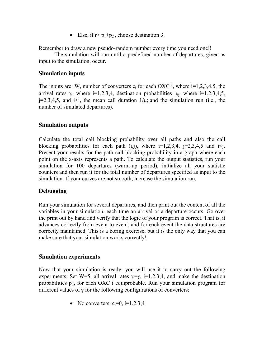Simulation experiments Now that your simulation is ready, you will use it to carry out the following experiments. Set W=5, all arrival rates γi=γ, i=1,2,3,4, and make the destination probabilities pij, for each OXC i equiprobable. 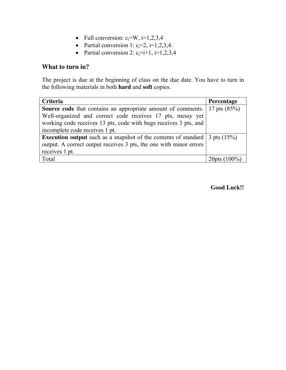Run your simulation program for different values of γ for the following configurations of converters: • No converters: ci=0, i=1,2,3,4 • Full conversion: ci=W, i=1,2,3,4 • Partial conversion 1: ci=2, i=1,2,3,4. • Partial conversion 2: ci=i+1, i=1,2,3,4 What to turn in? The project is due at the beginning of class on the due date. You have to turn in the following materials in both hard and soft copies. Criteria Percentage Source code that contains an appropriate amount of comments. Well-organized and correct code receives 17 pts, messy yet working code receives 13 pts, code with bugs receives 3 pts, and incomplete code receives 1 pt. 17 pts (85%) Execution output such as a snapshot of the contents of standard output. A correct output receives 3 pts, the one with minor errors receives 1 pt. 3 pts (15%) Total 20pts (100%) Good Luck!!