
CSC 422 Lecture Intensity Transform, Spring 2012
Notre Dame University–Louaize · Introduction to Image Processing · 32 pages · Dr. Khaldoun El-Khaldi



Showing the first 10 of 32 pages. Download the PDF to see all of it.
More CSC 422 files
Show the text of this lab
Intensity Transformations for
Image Enhancement
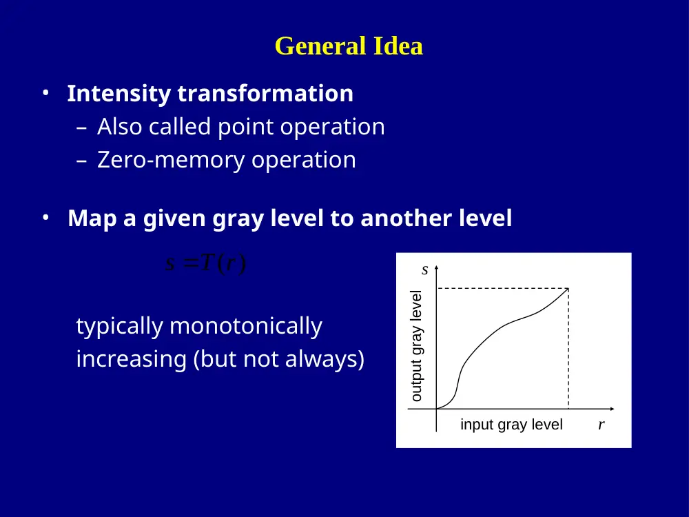
General Idea
• Intensity transformation
– Also called point operation
– Zero-memory operation
• Map a given gray level to another level
typically monotonically
increasing (but not always)
input gray level
r
output gray level
s
s T(r)
Intensity Histogram
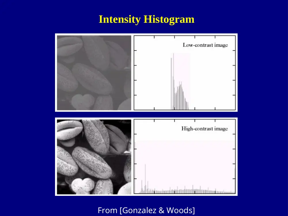
Intensity Histogram
1
3
8
6
6
8
6
11
8
10
8
9
9
7
10
10
0
1
2
3
4
k
6
7
8
9
10 11 12 13 14 15
0
1
0
1
0
0
3
1
4
2
3
1
0
0
0
0
5
H(k)
• Example
a 4x4, 4bits/pixel image
Intensity Histogram
From [Gonzalez & Woods]
Intensity Histogram
From [Gonzalez & Woods]
Fixed Intensity Transformations
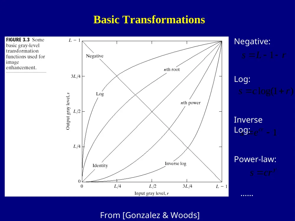
Basic Transformations
From [Gonzalez & Woods]
r
L
s
1
)
log(1
r
c
s
cr
s
Negative:
Log:
Power-law:
cr 1
e
s
Inverse
Log:
……
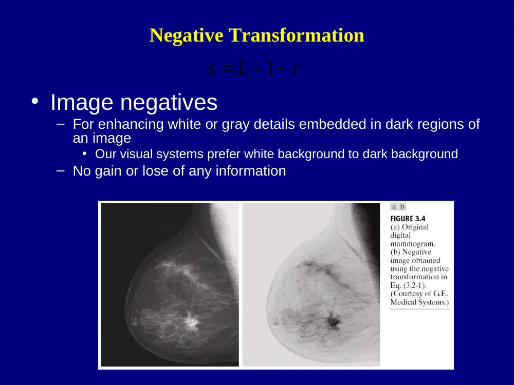
Negative Transformation
• Image negatives
– For enhancing white or gray details embedded in dark regions of
an image
• Our visual systems prefer white background to dark background
– No gain or lose of any information
r
L
s
1
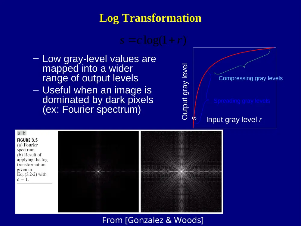
Log Transformation
– Low gray-level values are
mapped into a wider
range of output levels
– Useful when an image is
dominated by dark pixels
(ex: Fourier spectrum)
Input gray level r
Output gray level
s
Spreading gray levels
Compressing gray levels
From [Gonzalez & Woods]
)
log(1
r
c
s
Power-law (Gamma) Transformation
From [Gonzalez & Woods]
s cr
Power-law (Gamma) Transformation
From [Gonzalez & Woods]
s cr
Power-law (Gamma) Transformation
From [Gonzalez & Woods]
s cr
Application of Power Law Transformations
•
Gamma correction
– Many devices respond according to a power law
– Ex: The intensity-to-voltage response of a cathode ray tube (CRT)
m
r
if
m
if r
c
s
0
Thresholding
From [Gonzalez & Woods]
m : threshold
Example: Fixed Intensity Transformation
1
3
8
6
6
8
6
11
8
10
8
9
9
7
10
10
2
15
1
( )
r
round
T r
s
• A 4x4, 4bits/pixel image
passes through
an intensity transformation
0
1
4
2
2
4
2
8
4
7
4
5
5
3
7
7
1 round(0.0667) = 0;
3 round(0.6) = 1;
6 round(2.4) = 2;
7 round(3.2667) = 3;
8 round(4.2667) = 4;
9 round(5.4) =5;
10 round(6.6667) = 7;
11 round(8.0667) = 8;
The resulting
image is:
Example: Histogram Change
1
3
8
6
6
8
6
11
8
10
8
9
9
7
10
10
0
1
4
2
2
4
2
8
4
7
4
5
5
3
7
7
Contrast Stretch
General Idea: Make Best Use of the Dynamic Range
From [Gonzalez & Woods]
Contrast Stretch
min
max
min
)1
(2
r
r
r
r
s
B
1
2
1
2
)1
(2
1
2
1
2
0
2
2
2
2
2
2
2
1
1
2
2 1
2
1
1
2
1
2
1
1
1
B
B
B
B
B
r
r
r
r
s
r
r
s
r
r
r
r
r
s r
s r
r
r
r
s
s
r
r
r
r
s
s
max
2
r
r
General form:
Special case Full-scale contrast stretch:
min
1
r
r
1
2
2
B
s
1 0
s
min
max
min
)1
(2
r
r
r
r
round
s
B
Typically used:
Example: Full-Scale Contrast Stretch
4
4
8
6
6
8
6
11
8
11
8
8
9
7
10
10
min 4
r
0
0
9
4
4
9
4
15
9
15
9
9
11
6
13
13
• Full-scale contrast stretch
of a 4x4, 4bits/pixel image
• Find
rmax 11
15
1
2
B
4)
7 (
15
4
11
4
15
)1
2
(
min
max
min
r
round
r
round
r
r
r
r
round
s
B
4 round(0) = 0;
6 round(4.29) = 4;
7 round(6.43) = 6;
8 round(8.57) = 9;
9 round(10.71) = 11;
10 round(12.86) = 13;
11 round(15) = 15;
The resulting
image is:
Example: Histogram Change
4
4
8
6
6
8
6
11
8
11
8
8
9
7
10
10
0
0
9
4
4
9
4
15
9
15
9
9
11
6
13
13
Histogram Equalization
Histogram Equalization
From [Gonzalez & Woods]
Histogram Equalization
From [Gonzalez & Woods]
Example
2
3
8
2
9
9
9
10
8
3
3
8
3
11
11
10
min 2
r
0
2
10
0
12
12
12
13
10
2
2
10
2
15
15
13
• A 4x4, 4bits/pixel image
• First try: full-scale contrast stretch
max 11
r
2)
3 (
5
2
11
2
15
)1
2
(
min
max
min
r
round
r
round
r
r
r
r
round
s
B
2 round(0) = 0;
3 round(1.67) = 2;
8 round(10.00) = 10;
9 round(11.67) = 12;
10 round(13.33) = 13;
11 round(15) = 15;
The resulting
image is:
Example: Histogram Change
2
3
8
2
9
9
9
10
8
3
3
8
3
11
11
10
0
2
10
0
12
12
12
13
10
2
2
10
2
15
15
13
big gap
full-scale
contrast
stretch
original
Cumulative Histogram
0
1
2
3
4
k
6
7
8
9 10 11 12 13 14 15
0
0
2
4
0
0
0
0
3
3
2
2
0
0
0
0
5
H(k)
0
0
2
6
6
6
6
6
9 12 14 16 16 16 16 16
Q(k)
2
3
8
2
9
9
9
10
8
3
3
8
3
11
11
10
H(k)
Q(k)
Intermediate Image
2
3
8
2
9
9
9
10
8
3
3
8
3
11
11
10
2
6
9
2
12
12
12
14
9
6
6
9
6
16
16
14
0
1
2
3
4
k
6
7
8
9 10 11 12 13 14 15
0
0
2
4
0
0
0
0
3
3
2
2
0
0
0
0
5
H(k)
0
0
2
6
6
6
6
6
9 12 14 16 16 16 16 16
Q(k)
intermediate
image
original
2
6
9
2
12
12
12
14
9
6
6
9
6
16
16
14
min 2
r
0
4
8
0
11
11
11
13
8
4
4
8
4
15
15
13
max 16
r
2)
14 (
15
2
16
2
15
)1
2
(
min
max
min
r
round
r
round
r
r
r
r
round
s
B
2 round(0) = 0;
6 round(4.29) = 4;
9 round(7.50) = 8;
12 round(10.71) = 11;
14 round(12.86) = 13;
16 round(15) = 15;
final result:
histogram
equalized
image
Full-Scale Contrast Stretch of Intermediate Image
intermediat
e image
Histogram Comparison
4
4
8
6
6
8
6
11
8
11
8
8
9
7
10
10
0
4
8
0
11
11
11
13
8
4
4
8
4
15
15
13
0
2
10
0
12
12
12
13
10
2
2
10
2
15
15
13
original
direct full-scale contrast stretch
histogram-equalized
more
equalized
Summary of the Histogram Equalization Algorithm
original image
histogram H(k)
cumulative histogram Q(k)
intermediate image
full-scale contrast stretch
histogram-equalized image