CMPS 256 Midterm With Solution, Fall 2015

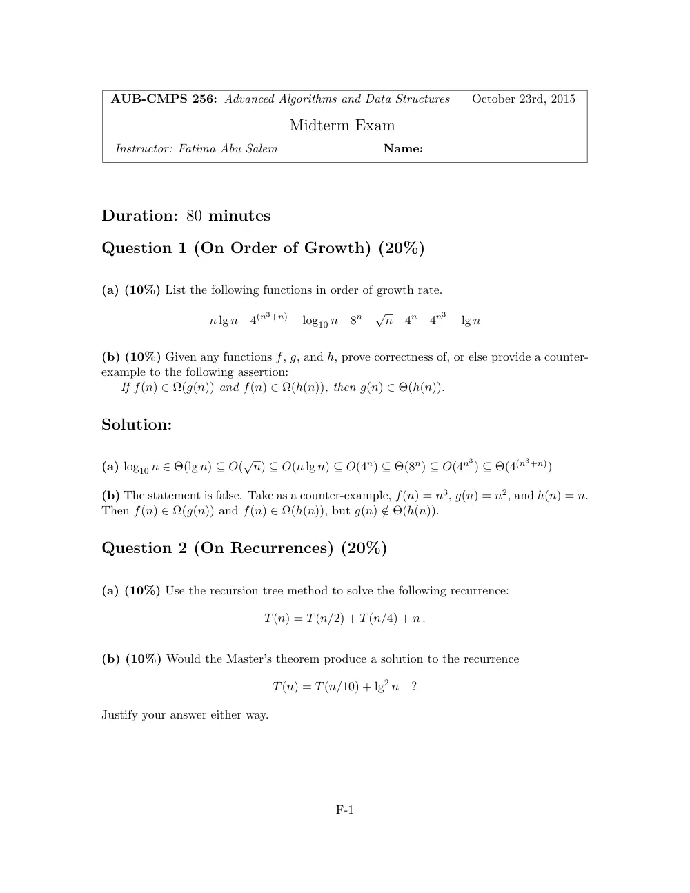
AUB-CMPS 256: Advanced Algorithms and Data Structures October 23rd, 2015 Midterm Exam Instructor: Fatima Abu Salem Name: Duration: 80 minutes Question 1 (On Order of Growth) (20%) (a) (10%) List the following functions in order of growth rate. n lg n 4(n3+n) log10 n 8n √n 4n 4n3 lg n (b) (10%) Given any functions f, g, and h, prove correctness of, or else provide a counter- example to the following assertion: If f(n) ∈ Ω(g(n)) and f(n) ∈ Ω(h(n)), then g(n) ∈ Θ(h(n)). Solution: (a) log10 n ∈ Θ(lg n) ⊆ O(√n) ⊆ O(n lg n) ⊆ O(4n) ⊆ Θ(8n) ⊆ O(4n3) ⊆ Θ(4(n3+n)) (b) The statement is false. Take as a counter-example, f(n) = n3, g(n) = n2, and h(n) = n. Then f(n) ∈ Ω(g(n)) and f(n) ∈ Ω(h(n)), but g(n) /∈ Θ(h(n)). Question 2 (On Recurrences) (20%) (a) (10%) Use the recursion tree method to solve the following recurrence: T(n) = T(n/2) + T(n/4) + n . (b) (10%) Would the Master’s theorem produce a solution to the recurrence T(n) = T(n/10) + lg2 n ? Justify your answer either way. 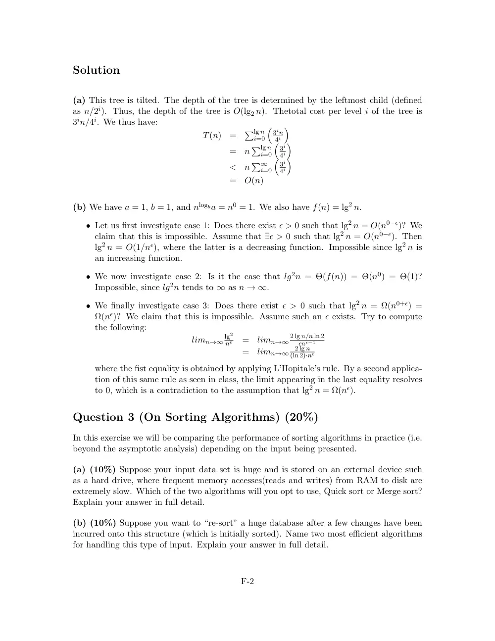F-1 Solution (a) This tree is tilted. The depth of the tree is determined by the leftmost child (defined as n/2i). Thus, the depth of the tree is O(lg2 n). Thetotal cost per level i of the tree is 3in/4i. We thus have: T(n) = �lg n i=0 � 3in 4i � = n �lg n i=0 � 3i 4i � < n �∞ i=0 � 3i 4i � = O(n) (b) We have a = 1, b = 1, and nlogba = n0 = 1. We also have f(n) = lg2 n. • Let us first investigate case 1: Does there exist ϵ > 0 such that lg2 n = O(n0−ϵ)? We claim that this is impossible. Assume that ∃ϵ > 0 such that lg2 n = O(n0−ϵ). Then lg2 n = O(1/nϵ), where the latter is a decreasing function. Impossible since lg2 n is an increasing function. • We now investigate case 2: Is it the case that lg2n = Θ(f(n)) = Θ(n0) = Θ(1)? Impossible, since lg2n tends to ∞ as n → ∞. • We finally investigate case 3: Does there exist ϵ > 0 such that lg2 n = Ω(n0+ϵ) = Ω(nϵ)? We claim that this is impossible. Assume such an ϵ exists. Try to compute the following: limn→∞ lg2 nϵ = limn→∞ 2 lg n/n ln 2 ϵnϵ−1 = limn→∞ 2 lg n (ln 2)·nϵ where the fist equality is obtained by applying L’Hopitale’s rule. By a second applica- tion of this same rule as seen in class, the limit appearing in the last equality resolves to 0, which is a contradiction to the assumption that lg2 n = Ω(nϵ). Question 3 (On Sorting Algorithms) (20%) In this exercise we will be comparing the performance of sorting algorithms in practice (i.e. beyond the asymptotic analysis) depending on the input being presented. (a) (10%) Suppose your input data set is huge and is stored on an external device such as a hard drive, where frequent memory accesses(reads and writes) from RAM to disk are extremely slow. Which of the two algorithms will you opt to use, Quick sort or Merge sort? Explain your answer in full detail. (b) (10%) Suppose you want to “re-sort” a huge database after a few changes have been incurred onto this structure (which is initially sorted). Name two most efficient algorithms for handling this type of input. Explain your answer in full detail. 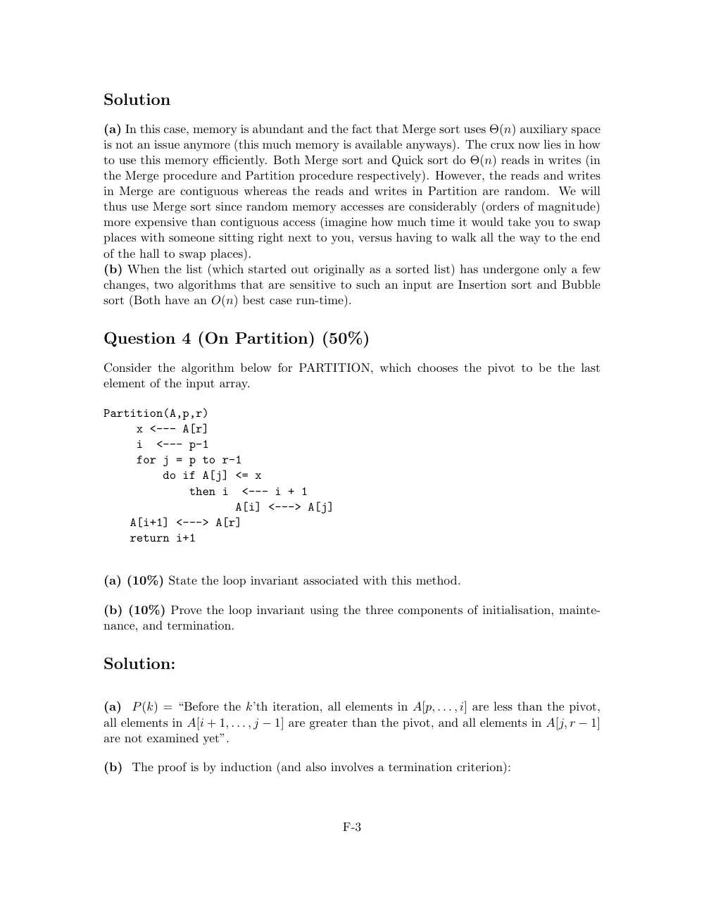F-2 Solution (a) In this case, memory is abundant and the fact that Merge sort uses Θ(n) auxiliary space is not an issue anymore (this much memory is available anyways). The crux now lies in how to use this memory efficiently. Both Merge sort and Quick sort do Θ(n) reads in writes (in the Merge procedure and Partition procedure respectively). However, the reads and writes in Merge are contiguous whereas the reads and writes in Partition are random. We will thus use Merge sort since random memory accesses are considerably (orders of magnitude) more expensive than contiguous access (imagine how much time it would take you to swap places with someone sitting right next to you, versus having to walk all the way to the end of the hall to swap places). (b) When the list (which started out originally as a sorted list) has undergone only a few changes, two algorithms that are sensitive to such an input are Insertion sort and Bubble sort (Both have an O(n) best case run-time). Question 4 (On Partition) (50%) Consider the algorithm below for PARTITION, which chooses the pivot to be the last element of the input array. Partition(A,p,r) x <--- A[r] i <--- p-1 for j = p to r-1 do if A[j] <= x then i <--- i + 1 A[i] <---> A[j] A[i+1] <---> A[r] return i+1 (a) (10%) State the loop invariant associated with this method. (b) (10%) Prove the loop invariant using the three components of initialisation, mainte- nance, and termination. Solution: (a) P(k) = “Before the k’th iteration, all elements in A[p, . . . , i] are less than the pivot, all elements in A[i + 1, . . . , j − 1] are greater than the pivot, and all elements in A[j, r − 1] are not examined yet”. 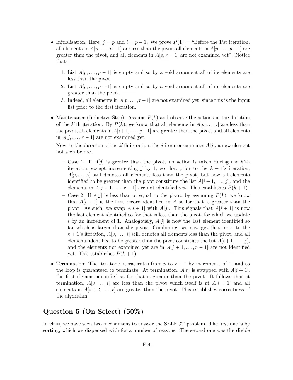(b) The proof is by induction (and also involves a termination criterion): F-3 • Initialisation: Here, j = p and i = p − 1. We prove P(1) = “Before the 1’st iteration, all elements in A[p, . . . , p−1] are less than the pivot, all elements in A[p, . . . , p−1] are greater than the pivot, and all elements in A[p, r − 1] are not examined yet”. Notice that: 1. List A[p, . . . , p − 1] is empty and so by a void argument all of its elements are less than the pivot. 2. List A[p, . . . , p − 1] is empty and so by a void argument all of its elements are greater than the pivot. 3. Indeed, all elements in A[p, . . . , r−1] are not examined yet, since this is the input list prior to the first iteration. • Maintenance (Inductive Step): Assume P(k) and observe the actions in the duration of the k’th iteration. By P(k), we know that all elements in A[p, . . . , i] are less than the pivot, all elements in A[i+1, . . . , j −1] are greater than the pivot, and all elements in A[j, . . . , r − 1] are not examined yet. Now, in the duration of the k’th iteration, the j iterator examines A[j], a new element not seen before. – Case 1: If A[j] is greater than the pivot, no action is taken during the k’th iteration, except incrementing j by 1, so that prior to the k + 1’s iteration, A[p, . . . , i] still denotes all elements less than the pivot, but now all elements identified to be greater than the pivot constitute the list A[i + 1, . . . , j], and the elements in A[j + 1, . . . , r − 1] are not identified yet. This establishes P(k + 1). – Case 2: If A[j] is less than or equal to the pivot, by assuming P(k), we know that A[i + 1] is the first record identified in A so far that is greater than the pivot. As such, we swap A[i + 1] with A[j]. This signals that A[i + 1] is now the last element identified so far that is less than the pivot, for which we update i by an increment of 1. Analogously, A[j] is now the last element identified so far which is larger than the pivot. Combining, we now get that prior to the k + 1’s iteration, A[p, . . . , i] still denotes all elements less than the pivot, and all elements identified to be greater than the pivot constitute the list A[i+1, . . . , j], and the elements not examined yet are in A[j + 1, . . . , r − 1] are not identified yet. This establishes P(k + 1). • Termination: The iterator j iteraterates from p to r − 1 by increments of 1, and so the loop is guaranteed to terminate. At termination, A[r] is swapped with A[i + 1], the first element identified so far that is greater than the pivot. It follows that at termination, A[p, . . . , i] are less than the pivot which itself is at A[i + 1] and all elements in A[i + 2, . . . , r] are greater than the pivot. This establishes correctness of the algorithm. Question 5 (On Select) (50%) In class, we have seen two mechanisms to answer the SELECT problem. The first one is by sorting, which we dispensed with for a number of reasons. The second one was the divide F-4 and conquer algorithm we named SELECT, with O(n) running time. 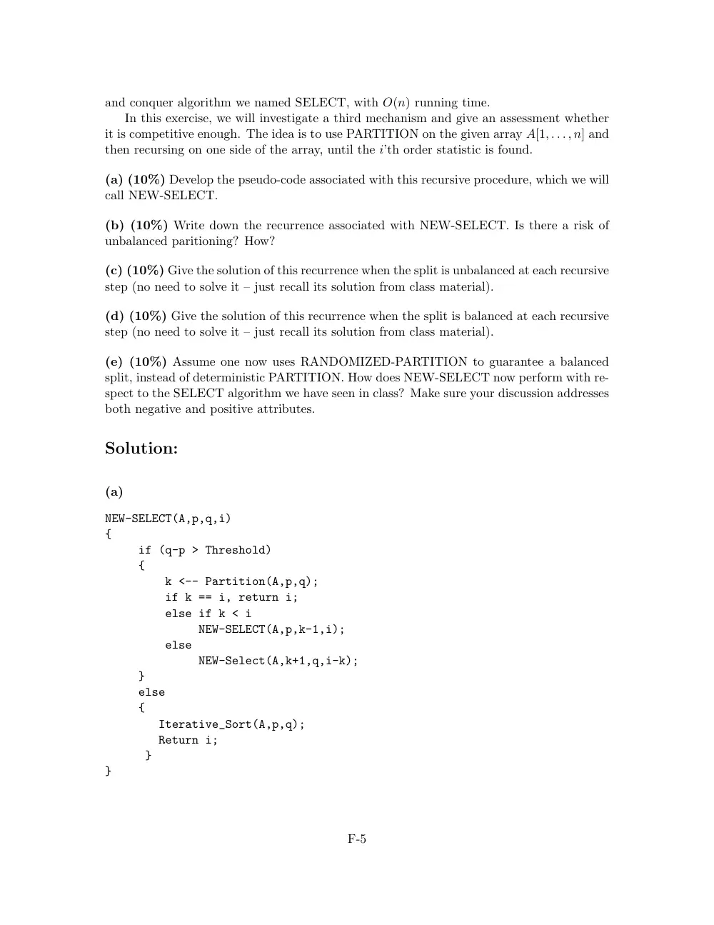In this exercise, we will investigate a third mechanism and give an assessment whether it is competitive enough. The idea is to use PARTITION on the given array A[1, . . . , n] and then recursing on one side of the array, until the i’th order statistic is found. (a) (10%) Develop the pseudo-code associated with this recursive procedure, which we will call NEW-SELECT. 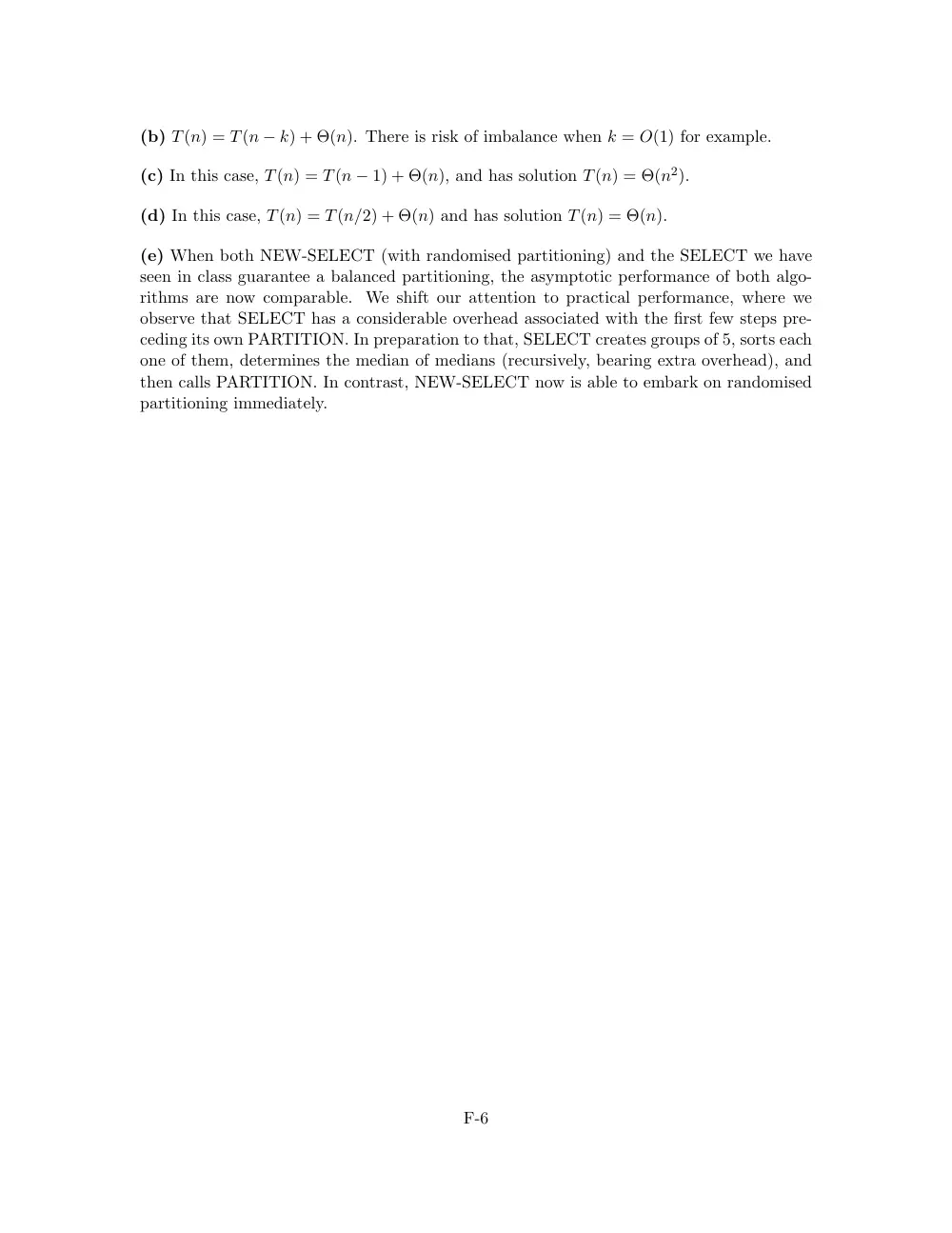(b) (10%) Write down the recurrence associated with NEW-SELECT. Is there a risk of unbalanced paritioning? How? (c) (10%) Give the solution of this recurrence when the split is unbalanced at each recursive step (no need to solve it – just recall its solution from class material). (d) (10%) Give the solution of this recurrence when the split is balanced at each recursive step (no need to solve it – just recall its solution from class material). (e) (10%) Assume one now uses RANDOMIZED-PARTITION to guarantee a balanced split, instead of deterministic PARTITION. How does NEW-SELECT now perform with re- spect to the SELECT algorithm we have seen in class? Make sure your discussion addresses both negative and positive attributes. Solution: (a) NEW-SELECT(A,p,q,i) { if (q-p > Threshold) { k <-- Partition(A,p,q); if k == i, return i; else if k < i NEW-SELECT(A,p,k-1,i); else NEW-Select(A,k+1,q,i-k); } else { Iterative_Sort(A,p,q); Return i; } } F-5 (b) T(n) = T(n − k) + Θ(n). There is risk of imbalance when k = O(1) for example. (c) In this case, T(n) = T(n − 1) + Θ(n), and has solution T(n) = Θ(n2). (d) In this case, T(n) = T(n/2) + Θ(n) and has solution T(n) = Θ(n). (e) When both NEW-SELECT (with randomised partitioning) and the SELECT we have seen in class guarantee a balanced partitioning, the asymptotic performance of both algo- rithms are now comparable. We shift our attention to practical performance, where we observe that SELECT has a considerable overhead associated with the first few steps pre- ceding its own PARTITION. In preparation to that, SELECT creates groups of 5, sorts each one of them, determines the median of medians (recursively, bearing extra overhead), and then calls PARTITION. In contrast, NEW-SELECT now is able to embark on randomised partitioning immediately. F-6