EECE 210C Lecture, Fall 2009

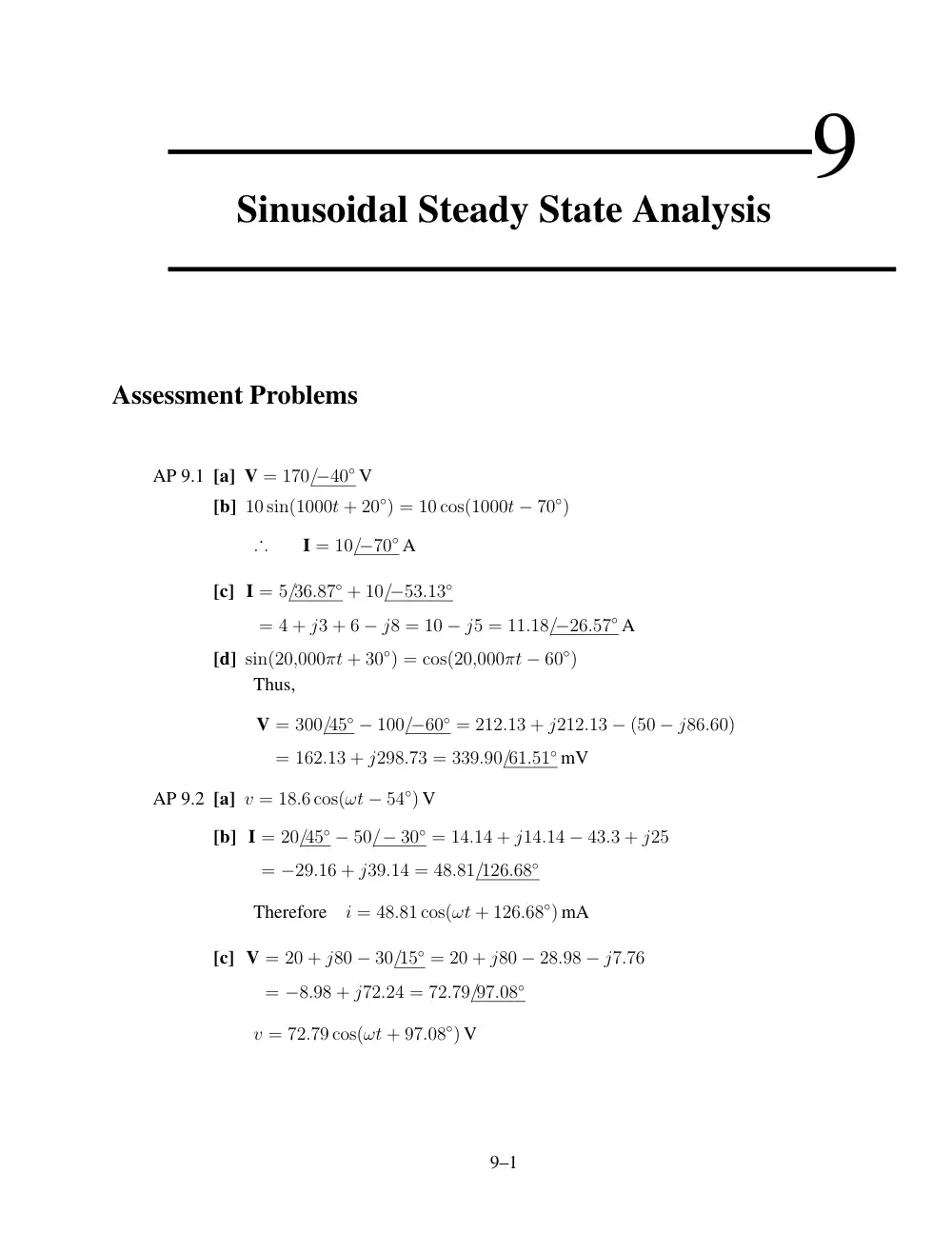
9 Sinusoidal Steady State Analysis Assessment Problems AP 9.1 [a] V = 170/−40◦ V [b] 10 sin(1000t + 20◦) = 10 cos(1000t − 70◦) ·. . I = 10/−70◦ A [c] I = 5/36.87◦ + 10/−53.13◦ = 4 + j3 + 6 − j8 = 10 − j5 = 11.18/−26.57◦ A [d] sin(20,000πt + 30◦) = cos(20,000πt − 60◦) Thus, V = 300/45◦ − 100/−60◦ = 212.13 + j212.13 − (50 − j86.60) = 162.13 + j298.73 = 339.90/61.51◦ mV AP 9.2 [a] v = 18.6 cos(ωt − 54◦) V [b] I = 20/45◦ − 50/− 30◦ = 14.14 + j14.14 − 43.3 + j25 = −29.16 + j39.14 = 48.81/126.68◦ Therefore i = 48.81 cos(ωt + 126.68◦) mA [c] V = 20 + j80 − 30/15◦ = 20 + j80 − 28.98 − j7.76 = −8.98 + j72.24 = 72.79/97.08◦ v = 72.79 cos(ωt + 97.08◦) V 9–1 9–2 CHAPTER 9. 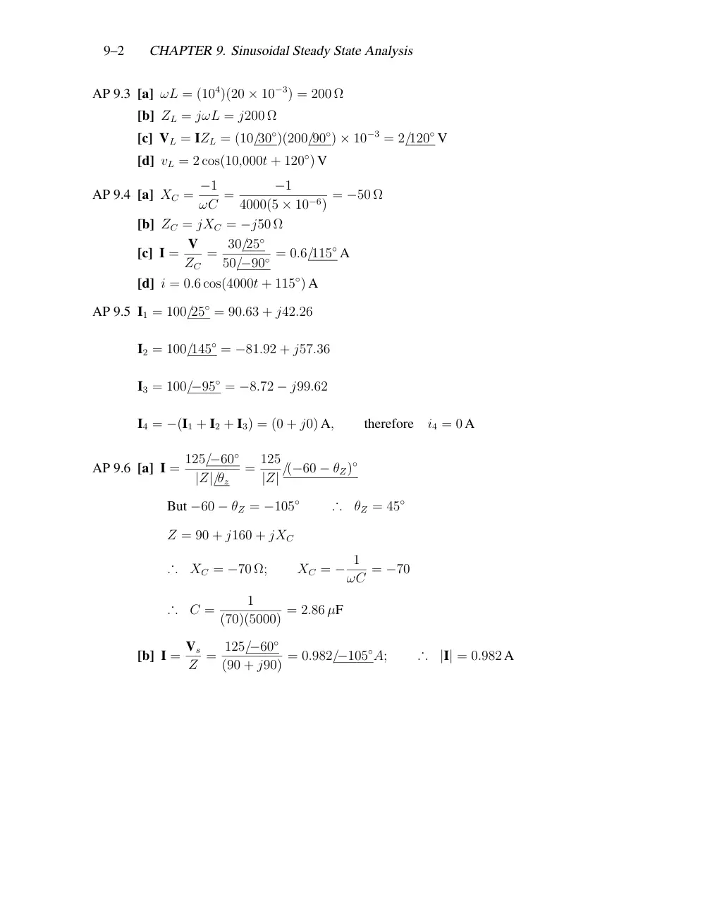Sinusoidal Steady State Analysis AP 9.3 [a] ωL = (104)(20 × 10−3) = 200 Ω [b] ZL = jωL = j200 Ω [c] VL = IZL = (10/30◦)(200/90◦) × 10−3 = 2/120◦ V [d] vL = 2 cos(10,000t + 120◦) V AP 9.4 [a] XC = −1 ωC = −1 4000(5 × 10−6) = −50 Ω [b] ZC = jXC = −j50 Ω [c] I = V ZC = 30/25◦ 50/−90◦ = 0.6/115◦ A [d] i = 0.6 cos(4000t + 115◦) A AP 9.5 I1 = 100/25◦ = 90.63 + j42.26 I2 = 100/145◦ = −81.92 + j57.36 I3 = 100/−95◦ = −8.72 − j99.62 I4 = −(I1 + I2 + I3) = (0 + j0) A, therefore i4 = 0 A AP 9.6 [a] I = 125/−60◦ |Z|/θz = 125 |Z| /(−60 − θZ)◦ But −60 − θZ = −105◦ ·. . θZ = 45◦ Z = 90 + j160 + jXC ·. . XC = −70 Ω; XC = − 1 ωC = −70 ·. . C = 1 (70)(5000) = 2.86 µF [b] I = Vs Z = 125/−60◦ (90 + j90) = 0.982/−105◦A; ·. . 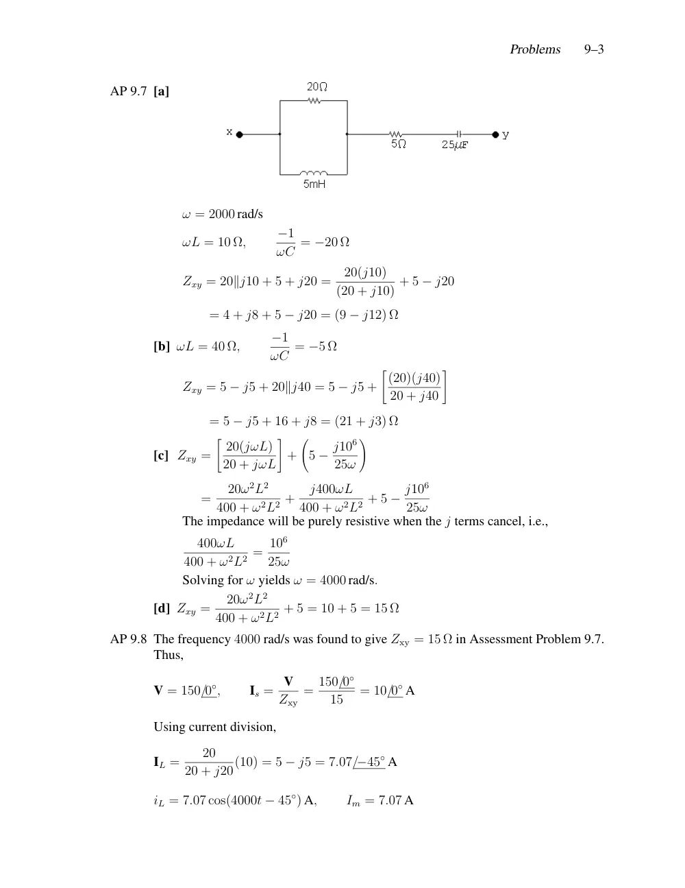|I| = 0.982 A Problems 9–3 AP 9.7 [a] ω = 2000 rad/s ωL = 10 Ω, −1 ωC = −20 Ω Zxy = 20∥j10 + 5 + j20 = 20(j10) (20 + j10) + 5 − j20 = 4 + j8 + 5 − j20 = (9 − j12) Ω [b] ωL = 40 Ω, −1 ωC = −5 Ω Zxy = 5 − j5 + 20∥j40 = 5 − j5 + �(20)(j40) 20 + j40 � = 5 − j5 + 16 + j8 = (21 + j3) Ω [c] Zxy = � 20(jωL) 20 + jωL � + � 5 − j106 25ω � = 20ω2L2 400 + ω2L2 + j400ωL 400 + ω2L2 + 5 − j106 25ω The impedance will be purely resistive when the j terms cancel, i.e., 400ωL 400 + ω2L2 = 106 25ω Solving for ω yields ω = 4000 rad/s. [d] Zxy = 20ω2L2 400 + ω2L2 + 5 = 10 + 5 = 15 Ω AP 9.8 The frequency 4000 rad/s was found to give Zxy = 15 Ω in Assessment Problem 9.7. Thus, V = 150/0◦, Is = V Zxy = 150/0◦ 15 = 10/0◦ A Using current division, IL = 20 20 + j20(10) = 5 − j5 = 7.07/−45◦ A iL = 7.07 cos(4000t − 45◦) A, Im = 7.07 A 9–4 CHAPTER 9. 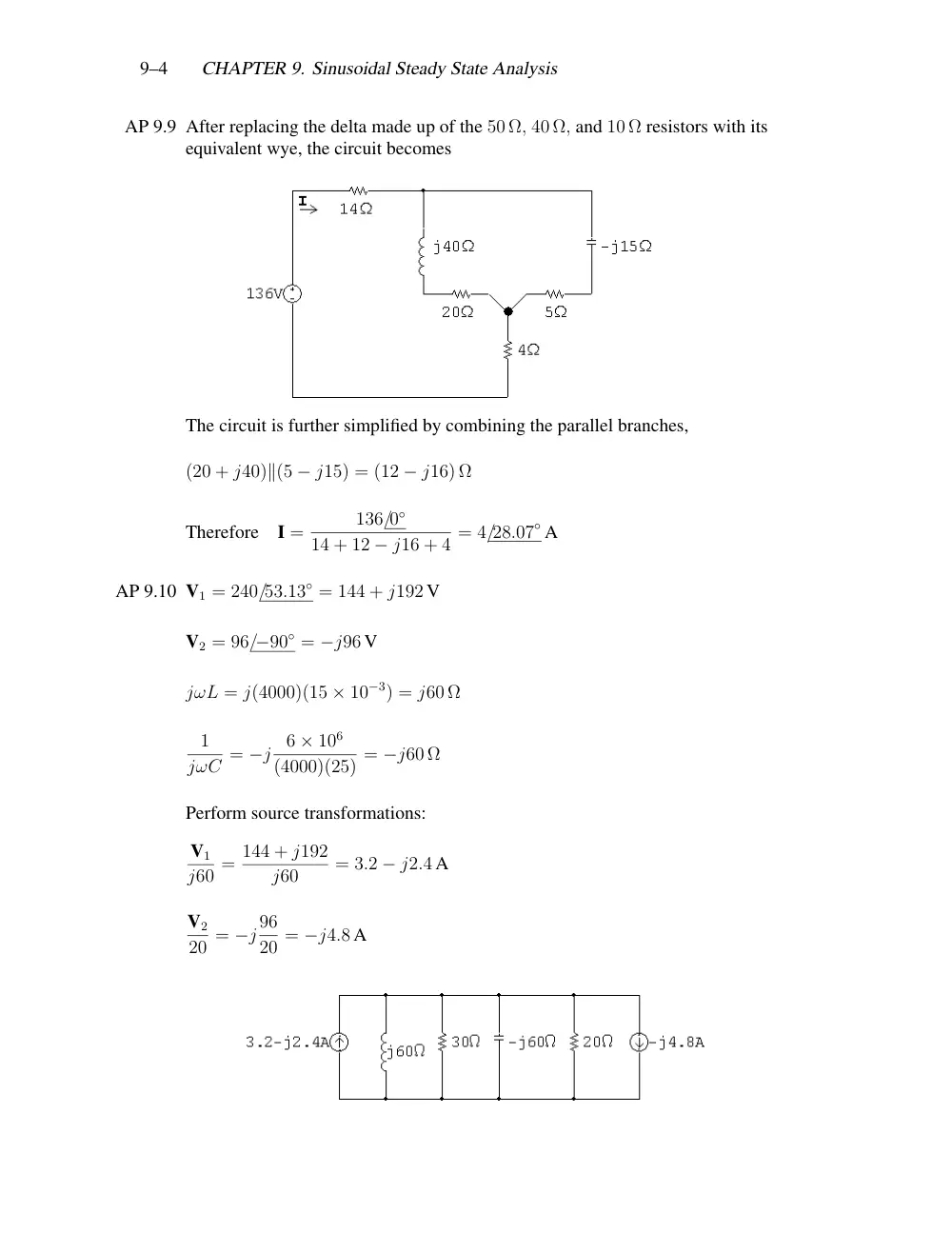Sinusoidal Steady State Analysis AP 9.9 After replacing the delta made up of the 50 Ω, 40 Ω, and 10 Ω resistors with its equivalent wye, the circuit becomes The circuit is further simplified by combining the parallel branches, (20 + j40)∥(5 − j15) = (12 − j16) Ω Therefore I = 136/0◦ 14 + 12 − j16 + 4 = 4/28.07◦ A AP 9.10 V1 = 240/53.13◦ = 144 + j192 V V2 = 96/−90◦ = −j96 V jωL = j(4000)(15 × 10−3) = j60 Ω 1 jωC = −j 6 × 106 (4000)(25) = −j60 Ω Perform source transformations: V1 j60 = 144 + j192 j60 = 3.2 − j2.4 A V2 20 = −j 96 20 = −j4.8 A Problems 9–5 Combine the parallel impedances: Y = 1 j60 + 1 30 + 1 −j60 + 1 20 = j5 j60 = 1 12 Z = 1 Y = 12 Ω 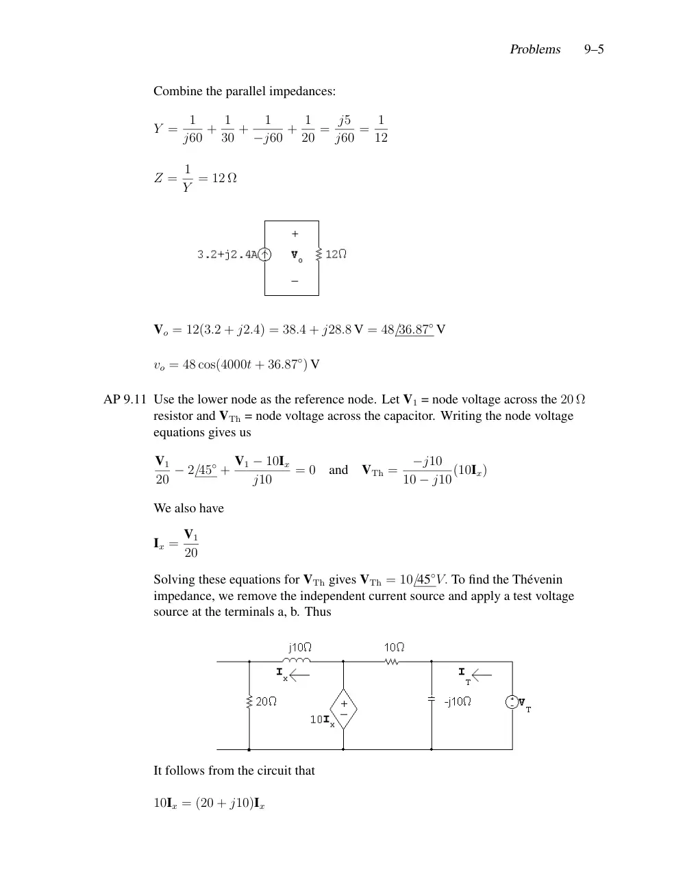Vo = 12(3.2 + j2.4) = 38.4 + j28.8 V = 48/36.87◦ V vo = 48 cos(4000t + 36.87◦) V AP 9.11 Use the lower node as the reference node. Let V1 = node voltage across the 20 Ω resistor and VTh = node voltage across the capacitor. Writing the node voltage equations gives us V1 20 − 2/45◦ + V1 − 10Ix j10 = 0 and VTh = −j10 10 − j10(10Ix) We also have Ix = V1 20 Solving these equations for VTh gives VTh = 10/45◦V. To find the Thévenin impedance, we remove the independent current source and apply a test voltage source at the terminals a, b. Thus It follows from the circuit that 10Ix = (20 + j10)Ix 9–6 CHAPTER 9. Sinusoidal Steady State Analysis Therefore Ix = 0 and IT = VT −j10 + VT 10 ZTh = VT IT , therefore ZTh = (5 − j5) Ω AP 9.12 The phasor domain circuit is as shown in the following diagram: The node voltage equation is −10 + V 5 + V −j(20/9) + V j5 + V − 100/−90◦ 20 = 0 Therefore V = 10 − j30 = 31.62/−71.57◦ Therefore v = 31.62 cos(50,000t − 71.57◦) V AP 9.13 Let Ia, Ib, and Ic be the three clockwise mesh currents going from left to right. Summing the voltages around meshes a and b gives 33.8 = (1 + j2)Ia + (3 − j5)(Ia − Ib) and 0 = (3 − j5)(Ib − Ia) + 2(Ib − Ic). But Vx = −j5(Ia − Ib), therefore Ic = −0.75[−j5(Ia − Ib)]. Solving for I = Ia = 29 + j2 = 29.07/3.95◦ A. 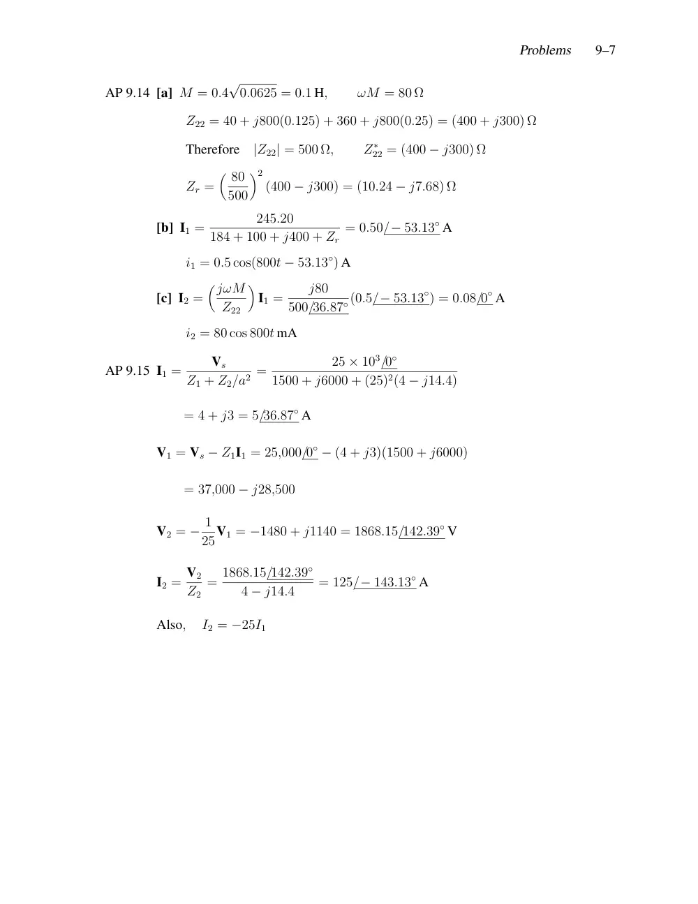Problems 9–7 AP 9.14 [a] M = 0.4 √ 0.0625 = 0.1 H, ωM = 80 Ω Z22 = 40 + j800(0.125) + 360 + j800(0.25) = (400 + j300) Ω Therefore |Z22| = 500 Ω, Z∗ 22 = (400 − j300) Ω Zr = � 80 500 �2 (400 − j300) = (10.24 − j7.68) Ω [b] I1 = 245.20 184 + 100 + j400 + Zr = 0.50/− 53.13◦ A i1 = 0.5 cos(800t − 53.13◦) A [c] I2 = �jωM Z22 � I1 = j80 500/36.87◦(0.5/− 53.13◦) = 0.08/0◦ A i2 = 80 cos 800t mA AP 9.15 I1 = Vs Z1 + Z2/a2 = 25 × 103/0◦ 1500 + j6000 + (25)2(4 − j14.4) = 4 + j3 = 5/36.87◦ A V1 = Vs − Z1I1 = 25,000/0◦ − (4 + j3)(1500 + j6000) = 37,000 − j28,500 V2 = − 1 25V1 = −1480 + j1140 = 1868.15/142.39◦ V I2 = V2 Z2 = 1868.15/142.39◦ 4 − j14.4 = 125/− 143.13◦ A Also, I2 = −25I1 9–8 CHAPTER 9. Sinusoidal Steady State Analysis Problems P 9.12 [a] 1000Hz [b] θv = 0◦ [c] I = 200/0◦ jωL = 200 ωL /− 90◦ = 25/− 90◦; θi = −90◦ [d] 200 ωL = 25; ωL = 200 25 = 8 Ω [e] L = 8 2π(1000) = 1.27 mH [f] ZL = jωL = j8 Ω P 9.13 [a] ω = 2πf = 314,159.27 rad/s [b] I = V ZC = 10 × 10−3/0◦ 1/jωC = jωC(10 × 10−3)/0◦ = 10 × 10−3ωC/90◦ ·. . θi = 90◦ [c] 628.32 × 10−6 = 10 × 10−3 ωC 1 ωC = 10 × 10−3 628.32 × 10−6 = 15.92 Ω, ·. . 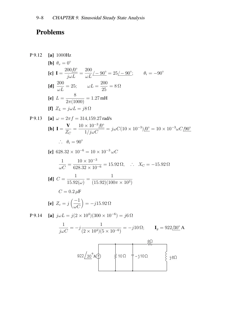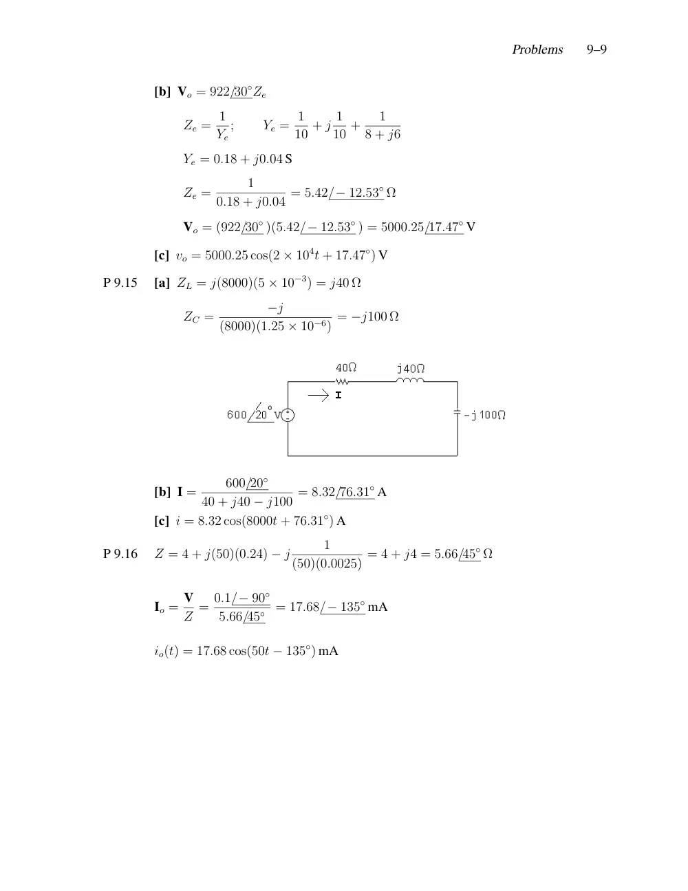XC = −15.92 Ω [d] C = 1 15.92(ω) = 1 (15.92)(100π × 103) C = 0.2 µF [e] Zc = j � −1 ωC � = −j15.92 Ω P 9.14 [a] jωL = j(2 × 104)(300 × 10−6) = j6 Ω 1 jωC = −j 1 (2 × 104)(5 × 10−6) = −j10 Ω; Ig = 922/30◦ A Problems 9–9 [b] Vo = 922/30◦Ze Ze = 1 Ye ; Ye = 1 10 + j 1 10 + 1 8 + j6 Ye = 0.18 + j0.04 S Ze = 1 0.18 + j0.04 = 5.42/− 12.53◦ Ω Vo = (922/30◦ )(5.42/− 12.53◦ ) = 5000.25/17.47◦ V [c] vo = 5000.25 cos(2 × 104t + 17.47◦) V P 9.15 [a] ZL = j(8000)(5 × 10−3) = j40 Ω ZC = −j (8000)(1.25 × 10−6) = −j100 Ω [b] I = 600/20◦ 40 + j40 − j100 = 8.32/76.31◦ A [c] i = 8.32 cos(8000t + 76.31◦) A P 9.16 Z = 4 + j(50)(0.24) − j 1 (50)(0.0025) = 4 + j4 = 5.66/45◦ Ω Io = V Z = 0.1/− 90◦ 5.66/45◦ = 17.68/− 135◦ mA io(t) = 17.68 cos(50t − 135◦) mA 9–10 CHAPTER 9. 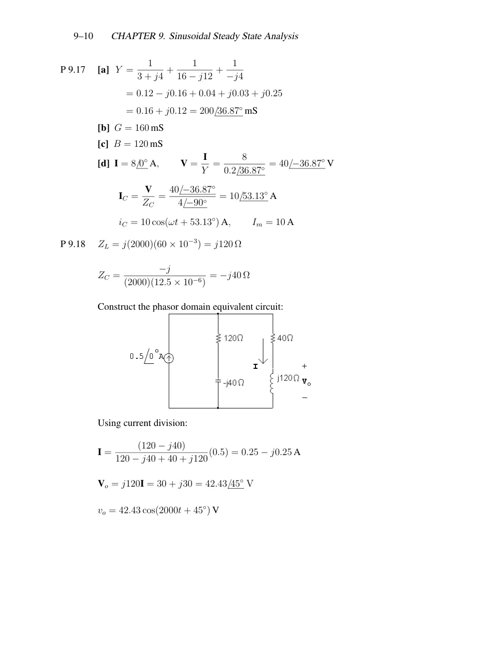Sinusoidal Steady State Analysis P 9.17 [a] Y = 1 3 + j4 + 1 16 − j12 + 1 −j4 = 0.12 − j0.16 + 0.04 + j0.03 + j0.25 = 0.16 + j0.12 = 200/36.87◦ mS [b] G = 160 mS [c] B = 120 mS [d] I = 8/0◦ A, V = I Y = 8 0.2/36.87◦ = 40/−36.87◦ V IC = V ZC = 40/−36.87◦ 4/−90◦ = 10/53.13◦ A iC = 10 cos(ωt + 53.13◦) A, Im = 10 A P 9.18 ZL = j(2000)(60 × 10−3) = j120 Ω ZC = −j (2000)(12.5 × 10−6) = −j40 Ω Construct the phasor domain equivalent circuit: Using current division: I = (120 − j40) 120 − j40 + 40 + j120(0.5) = 0.25 − j0.25 A Vo = j120I = 30 + j30 = 42.43/45◦ V vo = 42.43 cos(2000t + 45◦) V Problems 9–11 P 9.19 [a] Vg = 300/78◦; Ig = 6/33◦ ·. . Z = Vg Ig = 300/78◦ 6/33◦ = 50/45◦ Ω [b] ig lags vg by 45◦: 2πf = 5000π; f = 2500 Hz; T = 1/f = 400 µs ·. . ig lags vg by 45◦ 360◦(400 µs) = 50 µs P 9.20 1 jωC = 1 (1 × 10−6)(50 × 103) = −j20 Ω jωL = j50 × 103(1.2 × 10−3) = j60 Ω Vg = 40/0◦ V Ze = −j20 + 30∥j60 = 24 − j8 Ω Ig = 40/0◦ 24 − j8 = 1.5 + j0.5 mA Vo = (30∥j60)Ig = 30(j60) 30 + j60(1.5 + j0.5) = 30 + j30 = 42.43/45◦ V vo = 42.43 cos(50,000t + 45◦) V 9–12 CHAPTER 9. Sinusoidal Steady State Analysis P 9.35 Simplify the top triangle using series and parallel combinations: (1 + j1)∥(1 − j1) = 1 Ω Convert the lower left delta to a wye: Z1 = (j1)(1) 1 + j1 − j1 = j1 Ω Z2 = (−j1)(1) 1 + j1 − j1 = −j1 Ω Z3 = (j1)(−j1) 1 + j1 − j1 = 1 Ω Convert the lower right delta to a wye: Z4 = (−j1)(1) 1 + j1 − j1 = −j1 Ω Z5 = (−j1)(j1) 1 + j1 − j1 = 1 Ω Z6 = (j1)(1) 1 + j1 − j1 = j1 Ω The resulting circuit is shown below: Problems 9–13 Simplify the middle portion of the circuit by making series and parallel combinations: (1 + j1 − j1)∥(1 + 1) = 1∥2 = 2/3 Ω Zab = −j1 + 2/3 + j1 = 2/3 Ω P 9.39 Is = 3/0◦ mA 1 jωC = −j0.4 Ω jωL = j0.4 Ω After source transformation we have Vo = −j0.4∥j0.4∥5 28 + −j0.4∥j0.4∥5(66 × 10−3) = 10 mV vo = 10 cos 200t mV P 9.42 Using voltage division: VTh = 36 36 + j60 − j48(240) = 216 − j72 = 227.68/− 18.43◦ V Remove the source and combine impedances in series and in parallel: ZTh = 36∥(j60 − j48) = 3.6 + j10.8 Ω 9–14 CHAPTER 9. Sinusoidal Steady State Analysis P 9.43 Open circuit voltage: V2 10 + 88Iφ + V2 − 1 5V2 −j50 = 0 Iφ = 5 − (V2/5) 200 Solving, V2 = −66 + j88 = 110/126.87◦ V = VTh Find the Thévenin equivalent impedance using a test source: IT = VT 10 + 88Iφ + 0.8Vt −j50 Iφ = −VT/5 200 IT = VT � 1 10 − 881/5 200 + 0.8 −j50 � ·. . VT IT = 30 − j40 = ZTh IN = VTh ZTh = −66 + j88 30 − j40 = −2.2 + j0 A = 2.2/180◦ A Problems 9–15 The Norton equivalent circuit: P 9.51 V1 − 240 j10 + V1 50 + V1 30 + j10 = 0 Solving for V1 yields V1 = 198.63/− 24.44◦ V Vo = 30 30 + j10(V1) = 188.43/− 42.88◦ V P 9.54 The circuit with the mesh currents identified is shown below: 9–16 CHAPTER 9. Sinusoidal Steady State Analysis The mesh current equations are: −20/− 36.87◦ + j2I1 + 10(I1 − I2) = 0 50/− 106.26◦ + 10(I2 − I1) − j5I2 = 0 In standard form: I1(10 + j2) + I2(−10) = 20/− 36.87◦ I1(−10) + I2(10 − j5) = −50/− 106.26◦ = 50/73.74◦ Solving on a calculator yields: I1 = −6 + j10A; I2 = −9.6 + j10A Thus, Vo = 10(I1 − I2) = 36V and vo(t) = 36 cos 2000tV P 9.56 Write a KCL equation at the top node: Vo −j8 + Vo − 2.4I∆ j4 + Vo 5 − (10 + j10) = 0 The constraint equation is: I∆ = Vo −j8 Solving, Vo = j80 = 80/90◦ V Problems 9–17 P 9.59 (12 − j12)Ia − 12Ig − 5(−j8) = 0 −12Ia + (12 + j4)Ig + j20 − 5(j4) = 0 Solving, Ig = 4 − j2 = 4.47/− 26.57◦ A P 9.66 [a] jωL1 = j(5000)(2 × 10−3) = j10 Ω jωL2 = j(5000)(8 × 10−3) = j40 Ω jωM = j10 Ω 70 = (10 + j10)Ig + j10IL 0 = j10Ig + (30 + j40)IL Solving, Ig = 4 − j3 A; IL = −1 A ig = 5 cos(5000t − 36.87◦) A iL = 1 cos(5000t − 180◦) A 9–18 CHAPTER 9. Sinusoidal Steady State Analysis [b] k = M √L1L2 = 2 √ 16 = 0.5 [c] When t = 100π µs, 5000t = (5000)(100π) × 10−6 = 0.5π = π/2 rad = 90◦ ig(100πµs) = 5 cos(53.13◦) = 3 A iL(100πµs) = 1 cos(−90◦) = 0 A w = 1 2L1i2 1 + 1 2L2i2 2 + Mi1i2 = 1 2(2 × 10−3)(9) + 0 + 0 = 9 mJ When t = 200π µs, 5000t = π rad = 180◦ ig(200πµs) = 5 cos(180◦ − 36.87◦) = −4 A iL(200πµs) = 1 cos(180◦ − 180◦) = 1 A w = 1 2(2 × 10−3)(16) + 1 2(8 × 10−3)(1) + 2 × 10−3(−4)(1) = 12 mJ P 9.67 Remove the voltage source to find the equivalent impedance: ZTh = 45 + j125 + � 20 |5 + j5| �2 (5 − j5) = 85 + j85 Ω Using voltage division: VTh = Vcd = j20I1 = j20 � 425 5 + j5 � = 850 + j850 V = 1202.1/45◦ V Problems 9–19 P 9.71 ZL = V3 I3 = 80/60◦ Ω V2 10 = V3 1 ; 10I2 = 1I3 V1 8 = −V2 1 ; 8I1 = −1I2 Zab = V1 I1 Substituting, Zab = V1 I1 = −8V2 −I2/8 = 82V2 I2 = 82(10V3) I3/10 = (8)2(10)2V3 I3 = (8)2(10)2ZL = 512, 000/60◦ Ω