EECE 310L Report, Fall 2012

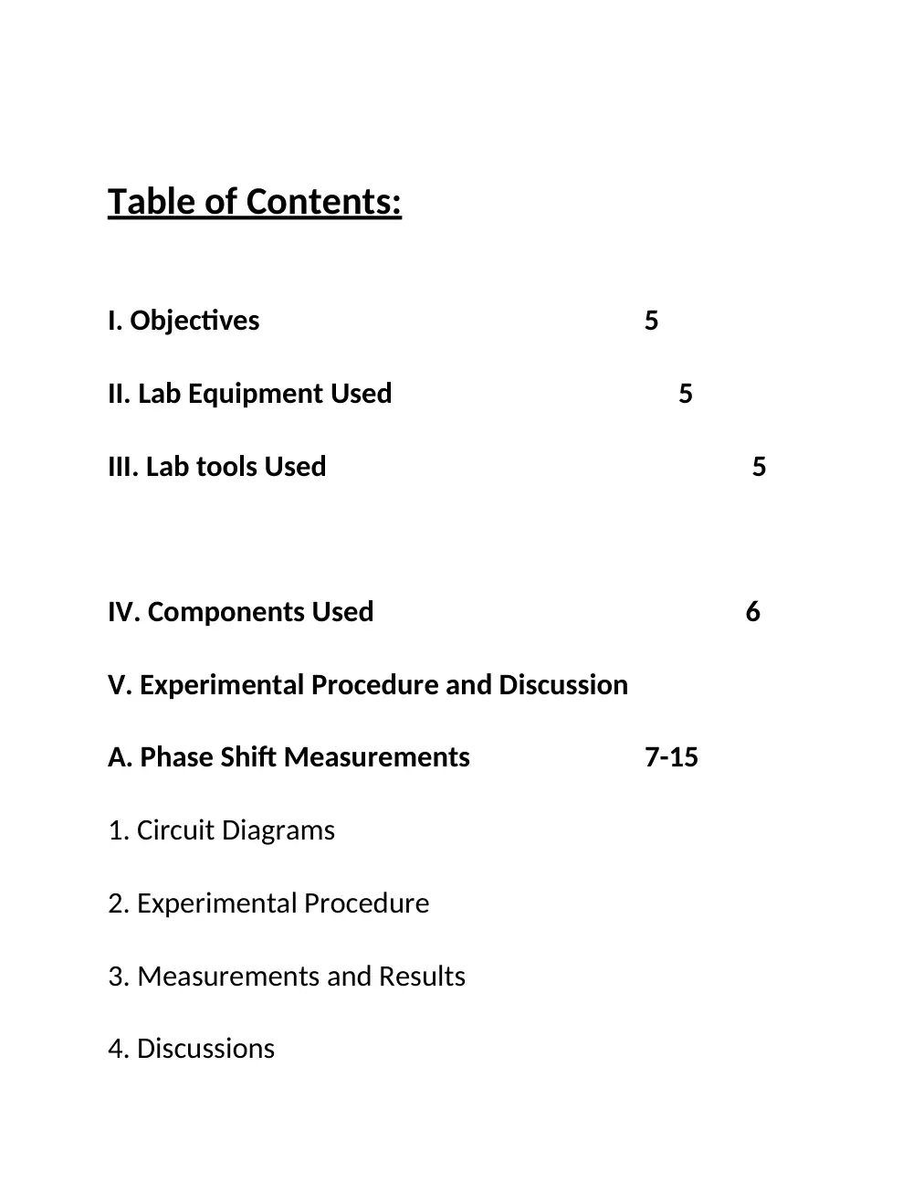
EECE 310 Lab Report for Experiment 4 Prepared by Yathreb El-Yaman 201204613 Yae11@aub.edu.lb Group 1, section 5 October 29 2012 RC and RLC Circuits Table of Contents: I. Objectives 5 II. Lab Equipment Used 5 III. Lab tools Used 5 IV. Components Used 6 V. Experimental Procedure and Discussion A. Phase Shift Measurements 7-15 1. Circuit Diagrams 2. Experimental Procedure 3. Measurements and Results 4. 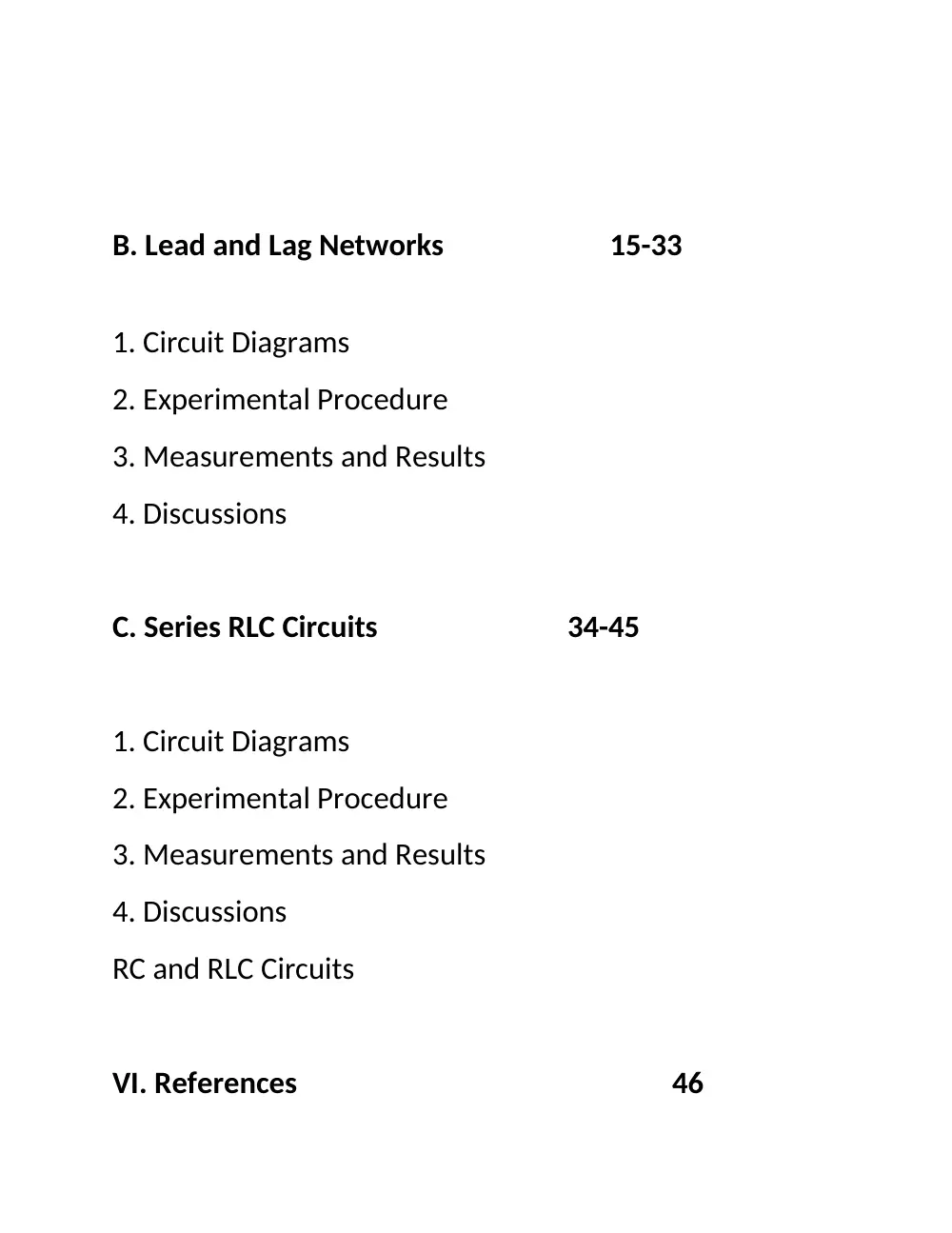Discussions B. Lead and Lag Networks 15-33 1. Circuit Diagrams 2. Experimental Procedure 3. Measurements and Results 4. Discussions C. Series RLC Circuits 34-45 1. Circuit Diagrams 2. Experimental Procedure 3. Measurements and Results 4. Discussions RC and RLC Circuits VI. 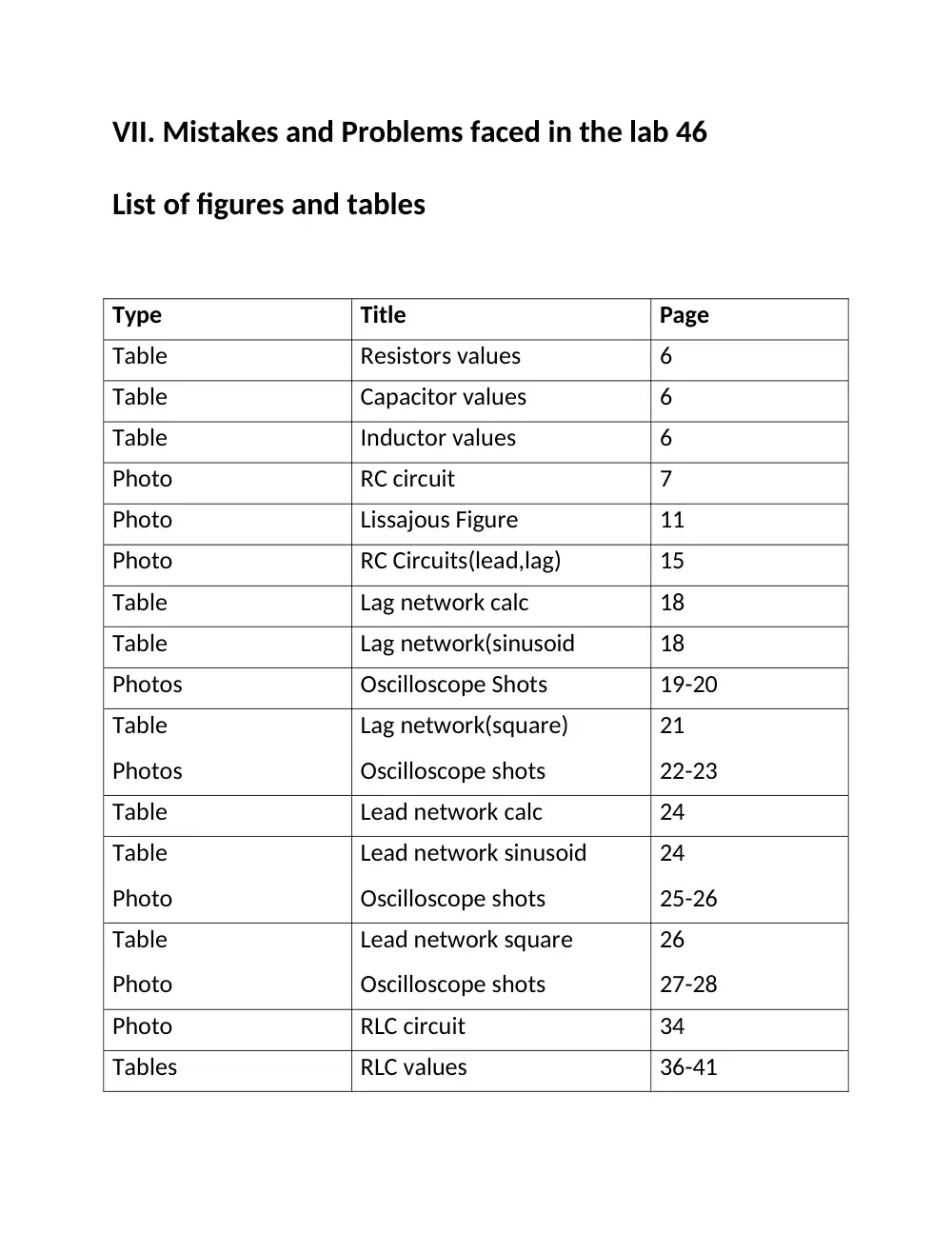References 46 VII. Mistakes and Problems faced in the lab 46 List of figures and tables Type Title Page Table Resistors values 6 Table Capacitor values 6 Table Inductor values 6 Photo RC circuit 7 Photo Lissajous Figure 11 Photo RC Circuits(lead,lag) 15 Table Lag network calc 18 Table Lag network(sinusoid 18 Photos Oscilloscope Shots 19-20 Table Photos Lag network(square) Oscilloscope shots 21 22-23 Table Lead network calc 24 Table Photo Lead network sinusoid Oscilloscope shots 24 25-26 Table Photo Lead network square Oscilloscope shots 26 27-28 Photo RLC circuit 34 Tables RLC values 36-41 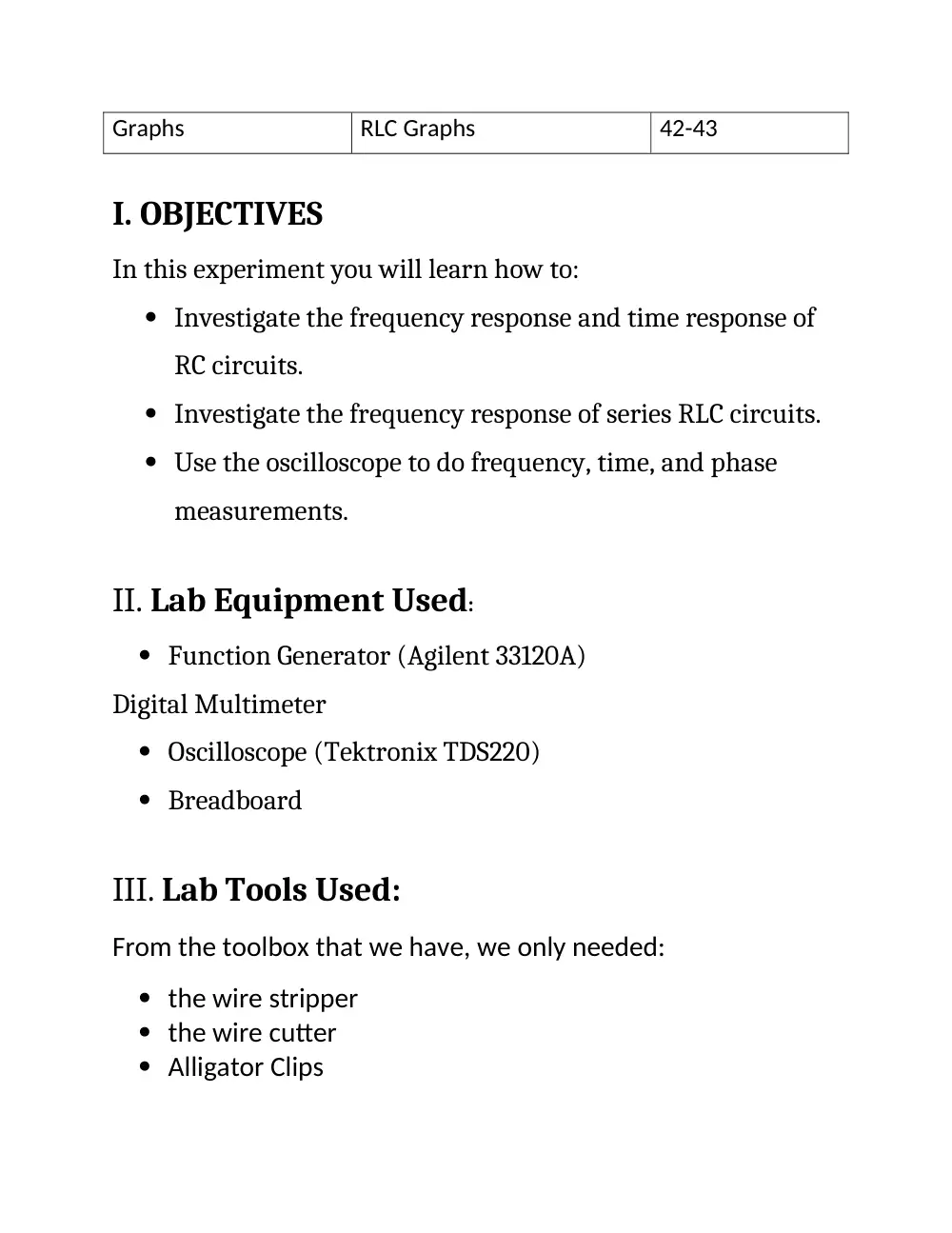Graphs RLC Graphs 42-43 I. OBJECTIVES In this experiment you will learn how to:  Investigate the frequency response and time response of RC circuits.  Investigate the frequency response of series RLC circuits.  Use the oscilloscope to do frequency, time, and phase measurements. II. Lab Equipment Used:  Function Generator (Agilent 33120A) Digital Multimeter  Oscilloscope (Tektronix TDS220)  Breadboard III. 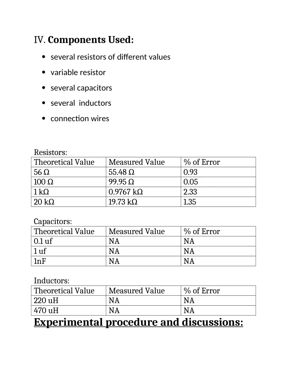Lab Tools Used: From the toolbox that we have, we only needed:  the wire stripper  the wire cutter  Alligator Clips IV. Components Used:  several resistors of different values  variable resistor  several capacitors  several inductors  connection wires Resistors: Theoretical Value Measured Value % of Error 56 Ω 55.48 Ω 0.93 100 Ω 99.95 Ω 0.05 1 kΩ 0.9767 kΩ 2.33 20 kΩ 19.73 kΩ 1.35 Capacitors: Theoretical Value Measured Value % of Error 0.1 uf NA NA 1 uf NA NA 1nF NA NA Inductors: Theoretical Value Measured Value % of Error 220 uH NA NA 470 uH NA NA Experimental procedure and discussions: 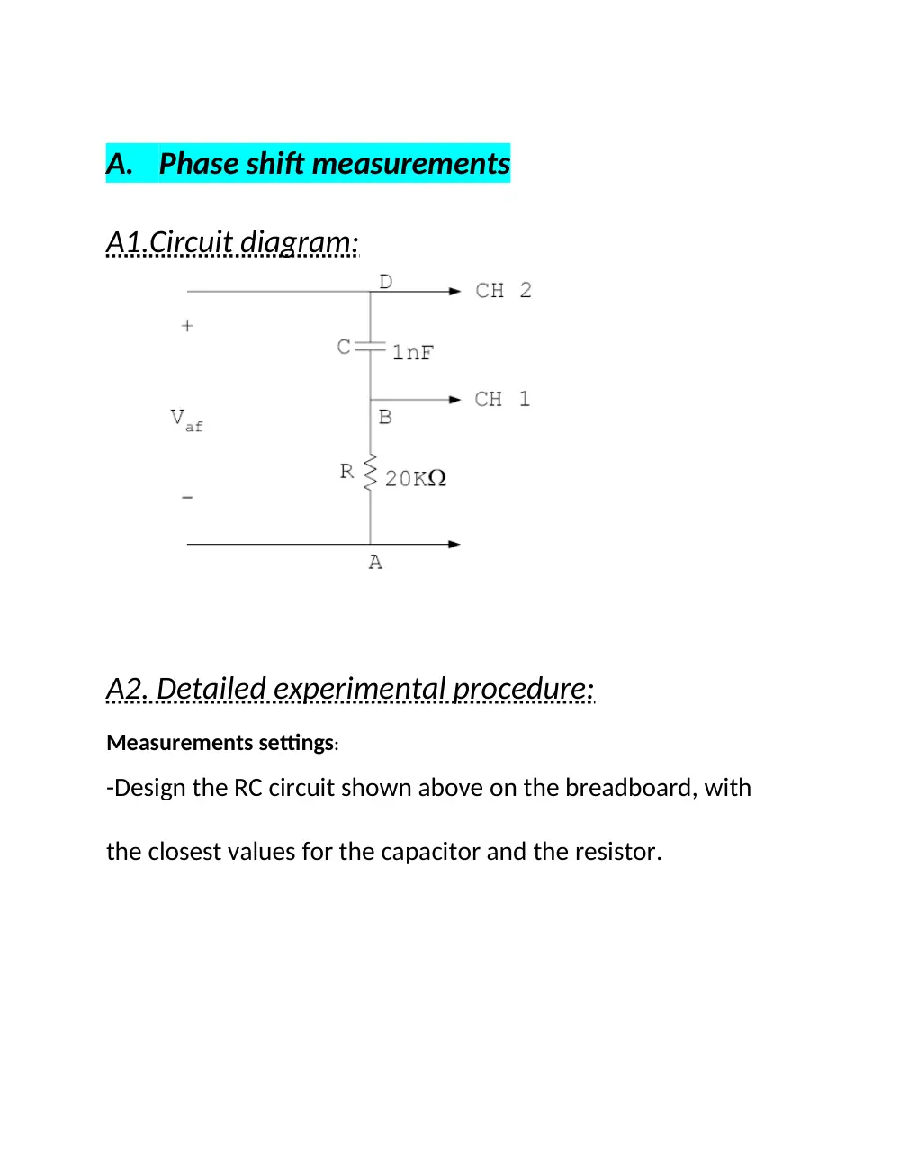A. Phase shift measurements A1.Circuit diagram: A2. Detailed experimental procedure: Measurements settings: -Design the RC circuit shown above on the breadboard, with the closest values for the capacitor and the resistor. 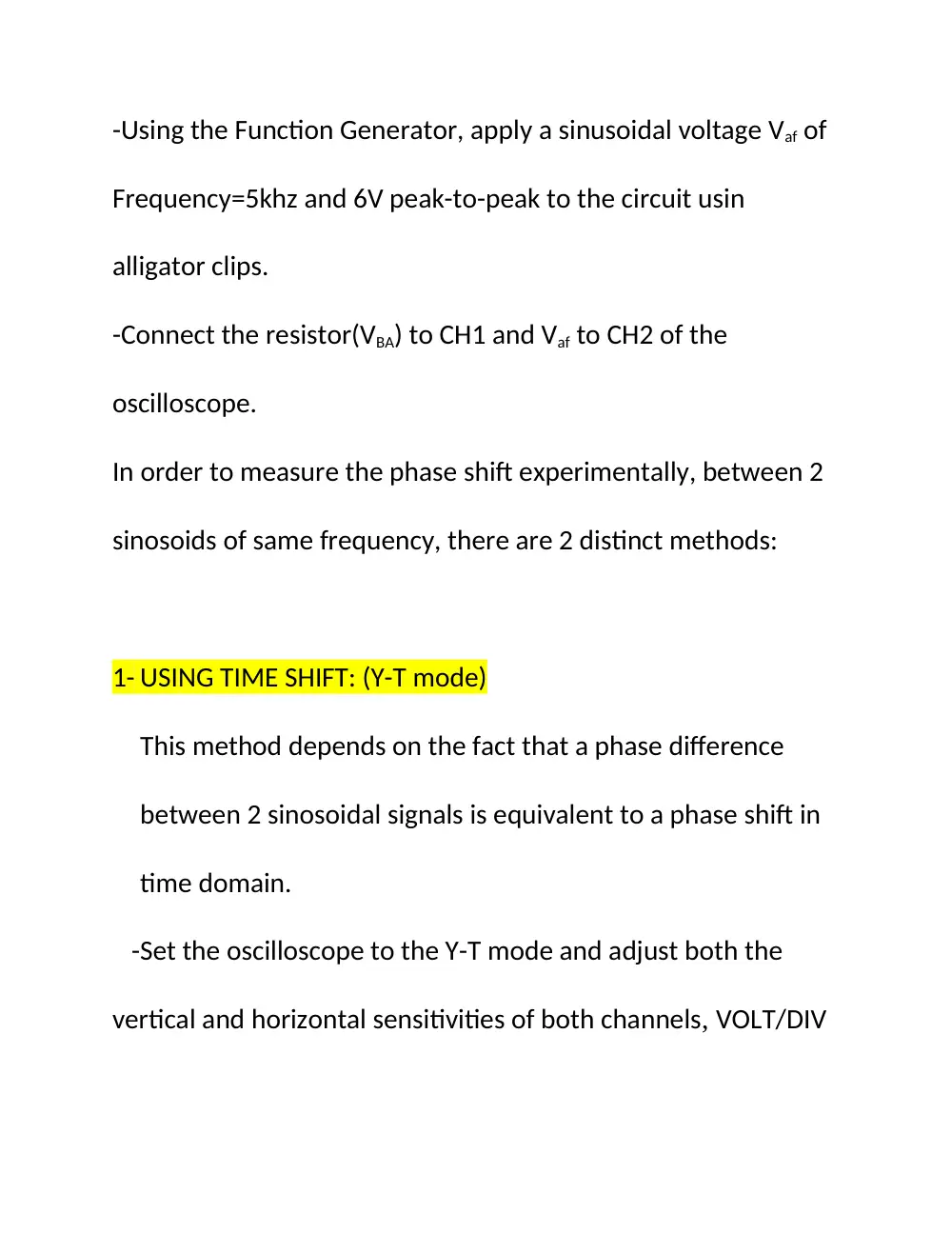-Using the Function Generator, apply a sinusoidal voltage Vaf of Frequency=5khz and 6V peak-to-peak to the circuit usin alligator clips. -Connect the resistor(VBA) to CH1 and Vaf to CH2 of the oscilloscope. In order to measure the phase shift experimentally, between 2 sinosoids of same frequency, there are 2 distinct methods: 1- USING TIME SHIFT: (Y-T mode) This method depends on the fact that a phase difference between 2 sinosoidal signals is equivalent to a phase shift in time domain. -Set the oscilloscope to the Y-T mode and adjust both the vertical and horizontal sensitivities of both channels, VOLT/DIV and SEC/DIV settings, to have them aligned and superposed on same horizontal axis. -Using the cursors measure the time difference ΔT between Vaf and VBA , set cursor 1 to the point where the signal 1 crosses the x-axis (or to an arbitrary point) and cursor 2 to the equivalent point on the second signal). ( choose the two closest peaks or two closest points where they cut x-axis). -Every one period in time domain is equivalent to 360o or 2π in angle domain, then: The phase angle φ= (ΔT/T)*360 in degrees, or φ= (ΔT/T)*2π in radians. Where T is the period of any of the signals(same frequency, same period) and ΔT is the time difference. Note that we can obtain T if we already know the frequency by simply using the formula: T= 1/F 2-USING LISSAJOUS FIGURE: (X-Y mode) -Set the oscilloscope to the X-Y mode and keep connections as in time shift method. -Lissajous method consists of measuring 2 parameters A and B from the ellipse shown on the. -VBA and VDA will be connected to the X and Y channels of the oscilloscope. -An ellipse (called the Lissajous figure) will be observed on the oscilloscope screen due to the superposition of two perpendicular sinusoids. -Center it using the vertical and horizontal POSITION knobs symmetrically w.r.t the origin. The centered ellipse will have the following shape: In this method the phase angle φ= sin-1(B/A) Assumptions: In this experiment the resistor used has 1.35% of error. In addition to the fact that wires have internal resistances. This fact is not taken into consideration during the theoretical calculations. A3. Measurements and results: Theoretical calculations: We can measure the phase angle using the following formula: Tan φ= Xc/R with Xc=1/(ωC) =1/ (2πfC) Given f= 5 kHz, R= 20 kΩ and C= 1nF Xc= 1/(2π*5*103*1*10-9)= 31847.134 Tan φ= 31847.134/20000=1.59 => φ= tan-11.59= 57.8o Experimental results: o Method 1: Y-T format Δ ΔT (s) T (s)=1/F Φ (degrees) 0.000032 0.0002 57.6 o Method 2: Lissajous figure 2B 2A Φ (degrees) 5.2 6 60 Comparison and %error: The theoretical value for this experiment is: 57.8o The experimental value obtained using the first method is: 57.6o The experimental value obtained using the second method is: 60o We can clearly see that, using the first method (time shift method) we obtained the closest value to the theoretical. But both errors are acceptable; that in addition to the errors of 5% range in the resistor and capacitor. In method 1, the percentage of error is: [(57.8-57.6)/57.8] *100 = .34% In method 2, the percentage of error is: [(57.8-60)/57.8] *100= 3.806% A4. Discussions: The shape of the ellipse depends on the frequency of the input.  At low frequencies, the capacitor acts as an open circuit, so VR=0 and so we observe either a vertical or horizontal straight line.  At very high frequencies, the ellipse looks like an oblique straight line which means that the capacitor acts as a short circuit and so Vout= Vin. phase shift=0 , VR directly proportional to current. This linearity is represented by a straight line in Lissajous Figure.  For the ellipse to be a Full circle, implies that we have A=B and so the phase angle = sin-1(1) = 90o. This occurs at very low frequencies. B. Lead and lag networks B1. Circuit diagram: B2. Detailed experimental procedure: Measurements settings: -Design the circuits above on the breadboard with the specified values of resistor and capacitor. The figure on the left is a lag network where Vout is on the capacitor, and the right figure represents a lead network where Vout is on the resistor. -Start with the lag network. And then with Lead network. -Connect Vin and Vout to the channels of oscilloscope. -Apply a sinusoidal signal, using function generator, of 1 V peak- to peak and of frequency initially 100Hz. We will vary it to 1000Hz(medium freq) and then to 10KHz(High freq) to observe the changes. -After finishing this experiment we will apply a square signal of same amplitude and same varied frequencies. o The magnitude of the transfer function of the lag network is: (VR is Vout and VSRC is Vin ) This means that Vout (peak to peak)= Vin *( 1 / √1+ω2C2R2) o The magnitude of the transfer function of lead network is: (VC is Vout and VSRC is Vin ) This means that Vout (peak to peak)= Vin *( ωCR / √1+ω2C2R2) Assumptions: In this experiment the resistor used has 2.33% of error. In addition to the fact that wires have internal resistances. This fact is not taken into consideration during the theoretical calculations. For LAG, having this transfer function, at high frequencies the output signal will be attenuated whereas at high frequencies the output signal is expected to be an exact replica of input. For LEAD, having that transfer function, at low frequencies the signal is attenuated while at high frequencies the output signal is an exact replica of the input one. B3. Measurements and results: FOR LAG: Sinusoidal wave: Theoretical calculations: Lag Network ( Calculated) Frequency Input Voltage Output Voltage VPk-Pk 100 Hz 1 VPk-Pk mVPk-Pk 1 KHz 1 VPk-Pk mVPk-Pk 10 KHz 1 VPk-Pk mVPk-Pk Experimental results: Lag Network ( Measured) Frequency Input Voltage Output Voltage VPk-Pk 100 Hz 1 VPk-Pk Vpp= mV pk-pk 1 KHz 1 VPk-Pk Vpp= mV pk-pk 998 846.73 157.17 1060 880 10 KHz 1 VPk-Pk Vpp= mV pk-pk The peak to peak values in the shots may be different to the stated measured values because they were varying and that could be due to noise in signal from the connection of wires.. For f = 100Hz, we obtained 2 overlapping graphs of Vout andVin 158 For f = 1 kHz. We can notice that Vout lags Vin. For f = 10KHz.We can notice that Vout clearly lags Vin in this case. Square wave: For the square wave input, we have the same calculated values as the sinusoidal wave. This is because we have the same transfer function independently of the signal nature. Experimental Results: Lag Network (Measured) Frequency Input Voltage Output Voltage VPk-Pk 100 Hz 1 VPk-Pk Vpp= mVPk-Pk 1 KHz 1 VPk-Pk Vpp= mVPk-Pk 10 KHz 1 VPk-Pk Vpp= mVPk-Pk For f = 100 Hz, 2 overlapping graphs of Vout andVin as shown in the figure 1080 1060 276 For f=1KHz. We observe distortion. For f=10KHz. Also more distortion closer to a sine wave. For LEAD: Sinosoidal Wave: Theoretical: Lead Network ( Calculated) Frequency Input Voltage Output Voltage VPk-Pk 100 Hz 1 VPk-Pk mVPk-Pk 1 KHz 1 VPk-Pk mVPk-Pk 10 KHz 1 VPk-Pk mVPk-Pk Experimental: Lead Network ( measured) Frequency Input Voltage Output Voltage VPk-Pk 100 Hz 1 VPk-Pk mVPk-Pk 1 KHz 1 VPk-Pk mVPk-Pk 10 KHz 1 VPk-Pk mVPk-Pk Lead 10KHz sine wave 62.7 530 1000 66 560 1020 Lead 1KHz sine wave Lead 100Hz sine wave SQUARE WAVE: Same theoretical as sinusoidal. Experimental: Lead Network ( Measured) Frequenc y Input Voltage Output Voltage VPk- Pk 100 Hz 1 VPk-Pk Vpp= V 1 KHz 1 VPk-Pk Vpp= V 10 KHz 1 VPk-Pk Vpp= V Lead square 10KHz. 2 overlapping graphs of Vout andVin Lead square 1KHz. Distortion. 1.78 1.96 1.32 Lead square 100Hz.low. the output appeared as steps and impulses… Comparison and error: Network Lag Lead Frequency( Hz) 100 1000 10000 100 1000 10000 Error % (sinosoids) 6.21 3.92 0.528 5.26 5.66 2 Error % (Square) 8.21 25.18 75.6 2738 269 32 B4. Discussions: LAG NETWORK: o At low Frequencies(100Hz), Vin=Vout.. The 2 graphs are overlapping. ( in phase) It is known that at low frequencies, the capacitor has enough time to charge up to a voltage = Vsource=Vin. o As we increase the frequency (period decreases), the capacitor does not have sufficient time to charge and discharge completely(capacitor doesn’t change its voltage instantaneously), and so it takes the shape seen in the figures of 1khz nad 10khz. -More attenuation -More phase shift -Amplitude decreases. IN square waves input, at high frequencies we will have distortion and not only attenuation. The sharp edges are built from highest frequencies.Those highest frequencies won’t pass due to the fact that the lag network is a low-pass filter distortion. o So to avoid attenuation of sinusoids, The frequency should be very low(f<<fc=1/RC) since a low pass filter(Lag network) attenuates the signal after its cut off frequency o Considering the fact that a square wave signal is a sum of sine waves at different frequencies, according to Fourier series expansion, whatever happens for sinosoids also applies to square waves o For lowest distortion, the fundamental frequency must be much less than the cut of frequency.(in both square and sign) o The lag network acts as an integrator at very high frequencies since H(s)=1/(1+sRC) approximately 1/sRC and that Laplace transform to time domain is equivalent to integration. Vc is the 1/C integral of I.  ,  This explains the shape of the graph of f=10Khz. Integral of square= triangular 2. LEAD NETWORK: For Square, The peak to peak value of output is greater than that of input due to the charging and discharging of the capacitor. since Vout=Vc+Vin . Vc charges till max  Vout=Vin+Vin=2Vin so peak of output could reach the value where its double that of input. o VR=RI=CdVc/dt At ω<<1/RC(very low frequencies  Capacitor has time to charge completely) Capacitor open circuit. Vc=Vin VR= CdVc/dt=RC dVin/dt  DIFFERENTIATOR. Or one can say, In lead network, H(s)=sRC/1+sRC = sRC and multiplying by s In Laplace is an equivalent differentiation in time domain. o So to avoid distortion of the square wave, the frequency should be very high(f>>fc=1/RC) so that more harmonics of the fourier series will be kept and thus the signal will be preserved. The Lead network is as a High pass filter that prevents the passage of low frequencies, frequencies less than the cut off freq. •f<<1/RC lead-network acts as a differentiator •f>> 1/RC  lag network acts as an integrator C.Series RLC Circuit C1. Circuit Diagram: C2. Detailed experimental procedure: Measurements settings: Setup the circuit shown above and connect VR and Vin to both channel of the oscilloscope. Sweep the frequency and measure the frequency with highest peak; this frequency is the resonant frequency, were the circuit is purely resistive. Also, measure the time shift between both signals. We provide a signal of 1 V peak to peak. Assumptions: Wires have internal resistances. This fact is not taken into consideration during the theoretical computations. C3. Measurements and results: Theoretical calculations: The Resonant frequency of an RLC circuit is: ωo= 1/ (2π√LC) (in Hz) or 0 = (in radians/ sec) The bandwidth of an RLC circuit is: BW= R/(2πL) (in Hz) or BW=R/L (in radians/ sec) Resistanc e Inducto r Capacito r Resonant Frequency Bandwidt h 100 Ω 220 µH 1 µf KHz KHz 10.73 72.379 56 Ω 220 µH 1 µf KHz KHz 100 Ω 470 µH 0.1 µf KHz KHz Experimental results: SET 1: SET 2: 10.73 40.532 7.341 33.879 SET 3: C4. Discussions: 1. For an RLC circuit, where the output is taken across R, the transfer function is: 2. for set 1: Frequen cy (Hz) | Vout/ Vin| Theoreti cal 1000 0.4375 0.5353 1400 0.6 0.6668 2000 0.695 0.793 2800 0.759 0.883 4000 0.815 0.946 5400 0.968 0.976 7500 0.936 0.994 10000 0.89 0.999 14000 0.907 0.9968 20000 0.9027 0.98 28000 0.8356 0.9496 40000 0.81 0.8898 54000 0.779 0.8127 75000 0.69 0.7016 100000 0.574 0.59 For set 2: Frequen cy (Hz) | Vout/ Vin| Theoreti cal 1000 0.448 0.539 1400 0.5778 0.674 2000 0.67 0.805 2800 0.7125 0.8995 4000 0.786 0.963 5400 0.813 0.99 7500 0.849 0.999 10000 0.808 0.99 14000 0.8 0.9579 20000 0.757 0.89 28000 0.71 0.792 40000 0.641 0.659 54000 0.536 0.538 75000 0.4299 0.4148 100000 0.345 0.322 For set 3: Frequen cy (Hz) | Vout/ Vin| Theoreti cal 1000 0.3 0.3345 1400 0.34 0.448 2000 0.45 0.589 2800 0.6 0.726 4000 0.69 0.853 5400 0.72 0.93 7500 0.79 0.9817 10000 0.8 0.999 14000 0.8 0.9899 20000 0.778 0.943 28000 0.72 0.8614 40000 0.672 0.737 54000 0.57 0.615 75000 0.468 0.428 100000 0.376 0.379 3. SET1: 1000 10000 100000 0 0.2 0.4 0.6 0.8 1 1.2 measured theoretical SET2: 1000 10000 100000 -1.11022302462516E-16 0.2 0.4 0.6 0.8 1 1.2 measured theoretical SET 3: 1000 10000 100000 0 0.2 0.4 0.6 0.8 1 1.2 measured theoretical 4.For each of graph we draw the line when the magnitude of transfer function is =1/. This line intersects the curves in two points f1 and f2 in which f2-f1 is the bandwidth. The resonant frequency is the frequency when the curves peak. - For set 1: BW=67.5Khz and F=1000Hz - For set 2: BW=25.2Khz and F=7500Hz - For set 3: BW=35Khz and F=1000Hz 5.Theoretical values: Resistanc Inducto Capacito Resonant Bandwidt e r r Frequency h 100 Ω 220 µH 1 µf KHz KHz 56 Ω 220 µH 1 µf KHz KHz 100 Ω 470 µH 0.1 µf KHz KHz There is a very notable difference between the two and this is due to the resistances present in the wires,components and misreading of the values from the graphs. 6. Since BW=R/2πL, the bandwidth and R are proportional. When R increases, BW increases, when R decreases BW decreases and vice versa. This is validated in the table where the 100ohm resistor gives a bandwidth greater that that of R=56ohms 10.73 72.379 10.73 40.532 7.341 33.879 7.Similarly, BW is inversely proportional to L, so as L increases or decreases BW decreases or increases respectively.(check sets 1 and 2) The bandwidth is independent of C. Thus the bandwidth isn’t affected by the change of C. 8. as seen in the table of question 5: Set 1 and set 3 have same resonant frequency (10.73) because they have same C and L. Set 2 has the lowest resonant frequency since the ratio of 1/radical LC is less thaan that of sets 1 and 3. Comparing sets 1 and 3,that have same R, The bandwidth of set 1 is the largest since it has lowest L whereas the bandwidth of set 2 is the narrowest (has biggest value of L). REFERENES: http://en.wikipedia.org/wiki/RC_circuit#Integrator Mistakes faced in Labs: No major conflicts were faced in the lab, other than some values in our measurements that weren’t stable due to connection errors. ------------------------------------------------------------------------------------------------------------------------------ “I HAVE NEITHER GIVEN NOR RECEIVED AID ON THIS REPORT NOR HAVE I CONCEALED ANY VIOLATION OF THE AUB STUDENT CODE OF CONDUCT.” Yathreb El_Yaman Yathreb El Yaman