EECE 471 Midterm, Fall 2006

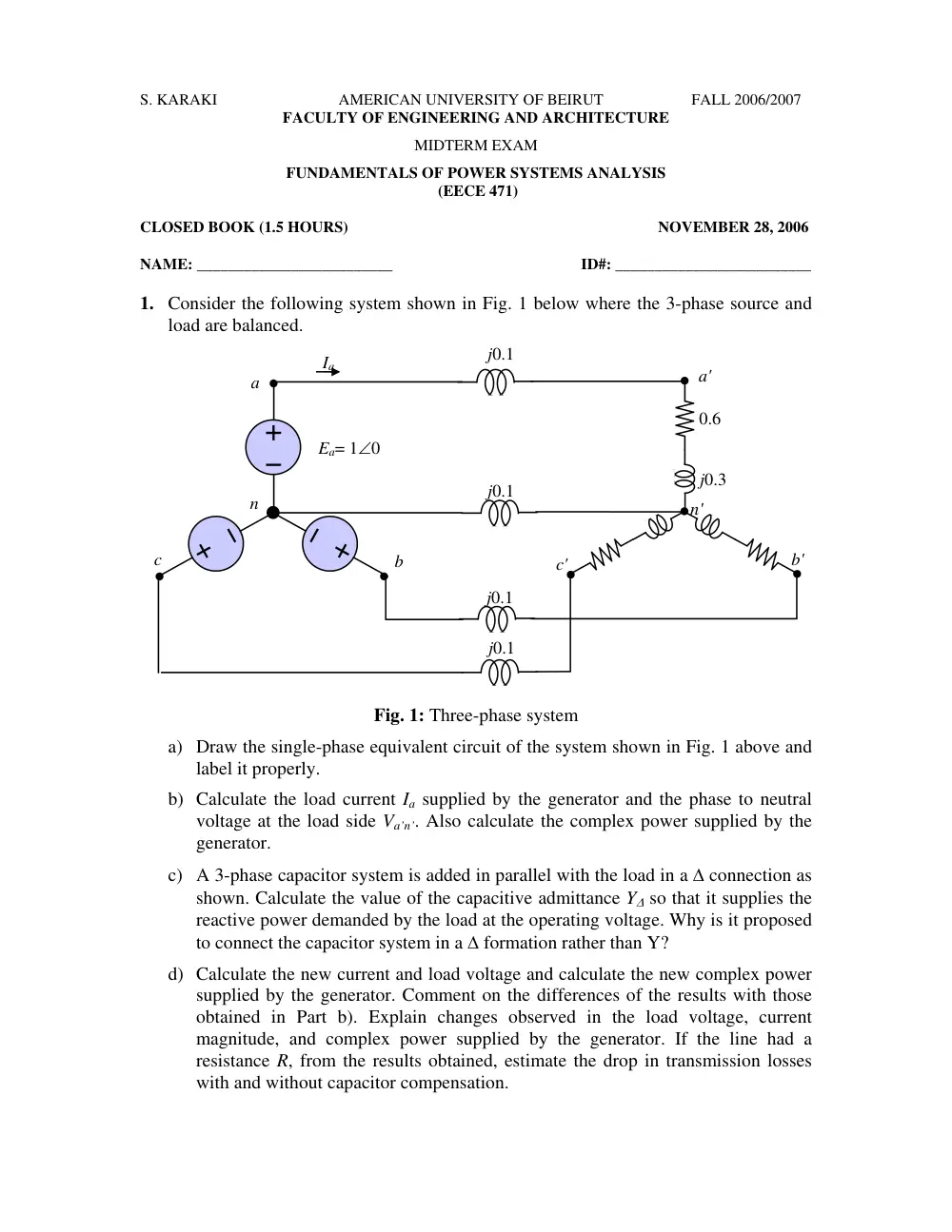
S. KARAKI AMERICAN UNIVERSITY OF BEIRUT FALL 2006/2007 FACULTY OF ENGINEERING AND ARCHITECTURE MIDTERM EXAM FUNDAMENTALS OF POWER SYSTEMS ANALYSIS (EECE 471) CLOSED BOOK (1.5 HOURS) NOVEMBER 28, 2006 NAME: _________________________ ID#: _________________________ 1. Consider the following system shown in Fig. 1 below where the 3-phase source and load are balanced. j0.1 j0.1 j0.1 j0.1 a b c Ia n a' c' j0.3 0.6 n' Ea= 1∠0 b' Fig. 1: Three-phase system a) Draw the single-phase equivalent circuit of the system shown in Fig. 1 above and label it properly. b) Calculate the load current Ia supplied by the generator and the phase to neutral voltage at the load side Va’n’. Also calculate the complex power supplied by the generator. c) A 3-phase capacitor system is added in parallel with the load in a ∆ connection as shown. Calculate the value of the capacitive admittance Y∆ so that it supplies the reactive power demanded by the load at the operating voltage. Why is it proposed to connect the capacitor system in a ∆ formation rather than Y? d) Calculate the new current and load voltage and calculate the new complex power supplied by the generator. Comment on the differences of the results with those obtained in Part b). Explain changes observed in the load voltage, current magnitude, and complex power supplied by the generator. If the line had a resistance R, from the results obtained, estimate the drop in transmission losses with and without capacitor compensation. EECE 471E MIDTERM - FALL 2006/ 07 Page 2/ 5 2. It is required to design a transmission line of 300 mile length to supply a demand of 250 MW at 0.9 PF lagging considering one of three voltages 132, 275 and 400 kV at a frequency of 50Hz with typical phase-to-phase spacing of 6, 10 m and 12 m, respectively. Note that 1 kcmil= 0.507mm2 and 1 ft= 0.305 m. 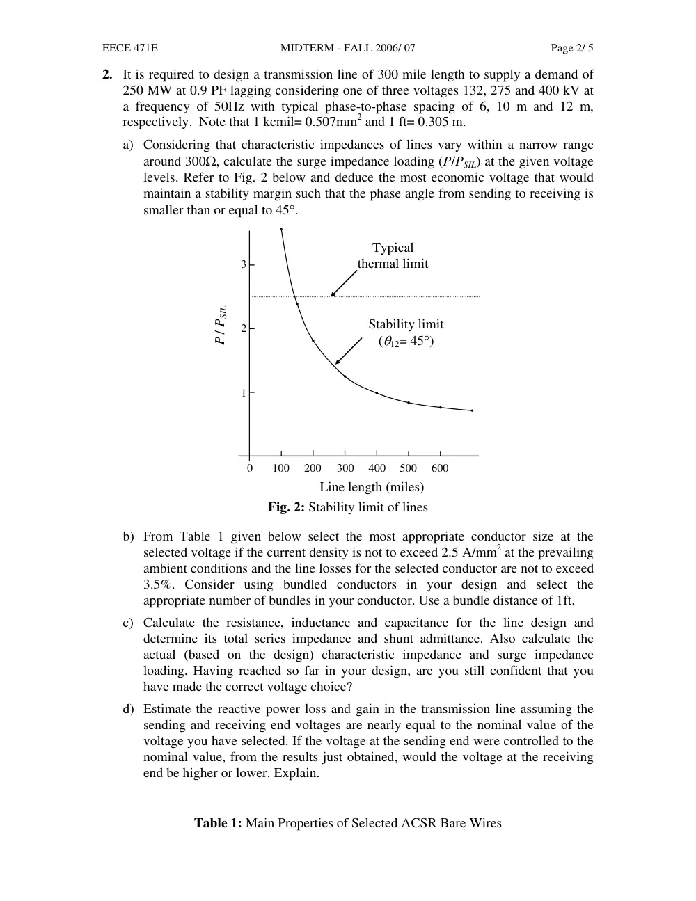a) Considering that characteristic impedances of lines vary within a narrow range around 300Ω, calculate the surge impedance loading (P/PSIL) at the given voltage levels. Refer to Fig. 2 below and deduce the most economic voltage that would maintain a stability margin such that the phase angle from sending to receiving is smaller than or equal to 45°. 100 200 300 400 500 600 0 1 2 3 P / PSIL Line length (miles) Typical thermal limit Stability limit (θ12= 45°) Fig. 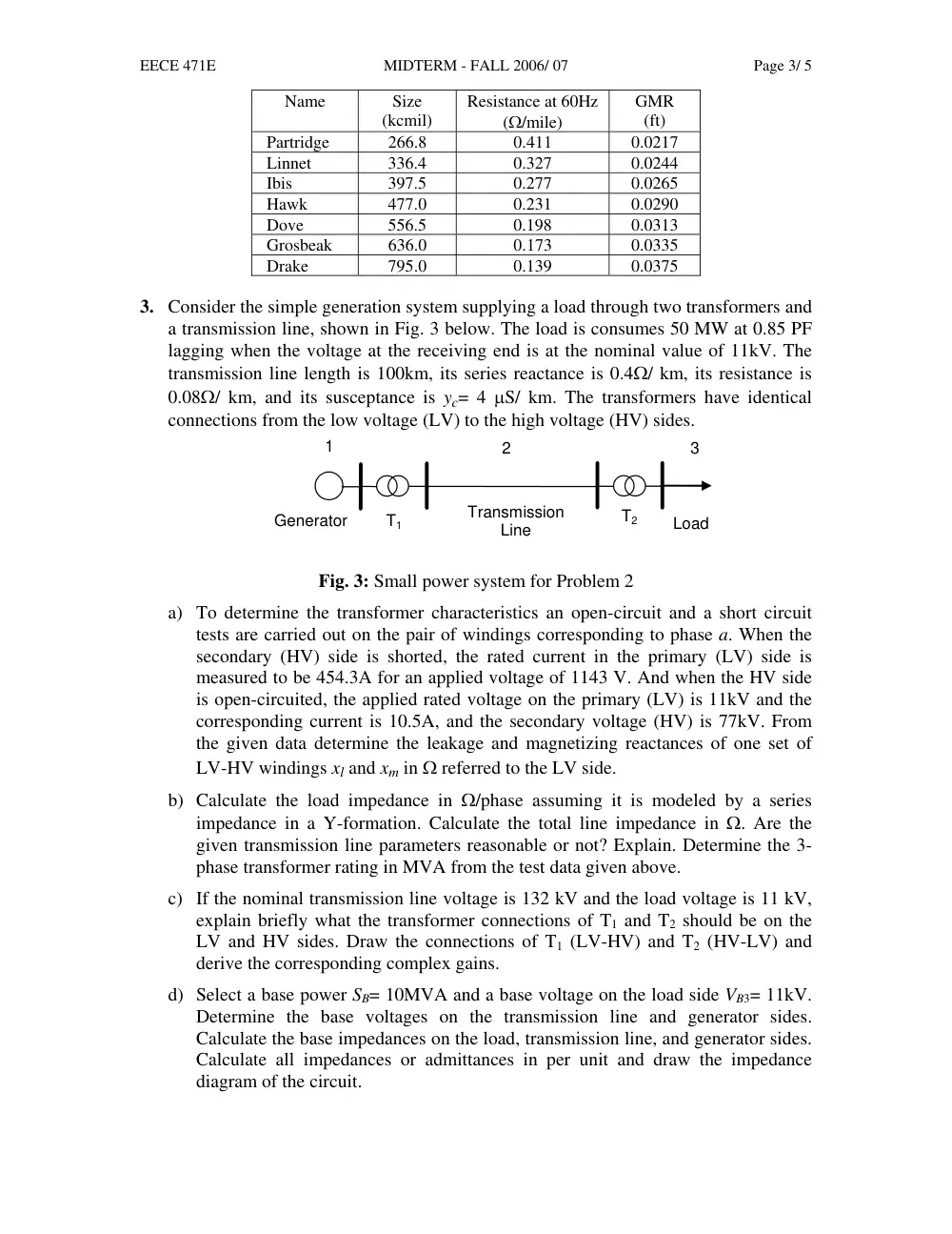2: Stability limit of lines b) From Table 1 given below select the most appropriate conductor size at the selected voltage if the current density is not to exceed 2.5 A/mm2 at the prevailing ambient conditions and the line losses for the selected conductor are not to exceed 3.5%. Consider using bundled conductors in your design and select the appropriate number of bundles in your conductor. Use a bundle distance of 1ft. c) Calculate the resistance, inductance and capacitance for the line design and determine its total series impedance and shunt admittance. Also calculate the actual (based on the design) characteristic impedance and surge impedance loading. Having reached so far in your design, are you still confident that you have made the correct voltage choice? d) Estimate the reactive power loss and gain in the transmission line assuming the sending and receiving end voltages are nearly equal to the nominal value of the voltage you have selected. If the voltage at the sending end were controlled to the nominal value, from the results just obtained, would the voltage at the receiving end be higher or lower. Explain. Table 1: Main Properties of Selected ACSR Bare Wires EECE 471E MIDTERM - FALL 2006/ 07 Page 3/ 5 Name Size (kcmil) Resistance at 60Hz (Ω/mile) GMR (ft) Partridge 266.8 0.411 0.0217 Linnet 336.4 0.327 0.0244 Ibis 397.5 0.277 0.0265 Hawk 477.0 0.231 0.0290 Dove 556.5 0.198 0.0313 Grosbeak 636.0 0.173 0.0335 Drake 795.0 0.139 0.0375 3. Consider the simple generation system supplying a load through two transformers and a transmission line, shown in Fig. 3 below. The load is consumes 50 MW at 0.85 PF lagging when the voltage at the receiving end is at the nominal value of 11kV. The transmission line length is 100km, its series reactance is 0.4Ω/ km, its resistance is 0.08Ω/ km, and its susceptance is yc= 4 µS/ km. The transformers have identical connections from the low voltage (LV) to the high voltage (HV) sides. Generator Load Transmission Line 1 2 3 T1 T2 Fig. 3: Small power system for Problem 2 a) To determine the transformer characteristics an open-circuit and a short circuit tests are carried out on the pair of windings corresponding to phase a. When the secondary (HV) side is shorted, the rated current in the primary (LV) side is measured to be 454.3A for an applied voltage of 1143 V. And when the HV side is open-circuited, the applied rated voltage on the primary (LV) is 11kV and the corresponding current is 10.5A, and the secondary voltage (HV) is 77kV. From the given data determine the leakage and magnetizing reactances of one set of LV-HV windings xl and xm in Ω referred to the LV side. b) Calculate the load impedance in Ω/phase assuming it is modeled by a series impedance in a Y-formation. Calculate the total line impedance in Ω. Are the given transmission line parameters reasonable or not? Explain. Determine the 3- phase transformer rating in MVA from the test data given above. c) If the nominal transmission line voltage is 132 kV and the load voltage is 11 kV, explain briefly what the transformer connections of T1 and T2 should be on the LV and HV sides. Draw the connections of T1 (LV-HV) and T2 (HV-LV) and derive the corresponding complex gains. d) Select a base power SB= 10MVA and a base voltage on the load side VB3= 11kV. Determine the base voltages on the transmission line and generator sides. Calculate the base impedances on the load, transmission line, and generator sides. Calculate all impedances or admittances in per unit and draw the impedance diagram of the circuit. 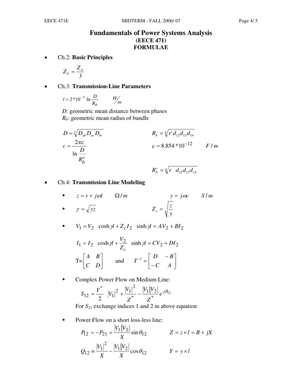EECE 471E MIDTERM - FALL 2006/ 07 Page 4/ 5 Fundamentals of Power Systems Analysis (EECE 471) FORMULAE • Ch.2: Basic Principles 3 ZY = Z∆ • Ch.3: Transmission-Line Parameters H m R D l b ln 2*10 −7 = D: geometric mean distance between phases Rb: geometric mean radius of bundle 3 bc ac ab D D D D = 4 14 ' 12 13 r d d d Rb = c b R D c ln = 2πε F / m .8 854*10 −12 ε = 4 14 12 13 r d d d R c b = • Ch.4: Transmission Line Modeling � m j l r z Ω / + = ω S m j c y / = ω � yz γ = y z Z c = � 2 2 2 2 1 sinh cosh BI AV l Z I l V V c + = + = γ γ 2 2 2 2 1 sinh cosh DI CV l Z V l I I c + = + = γ γ T= ⎥⎦ ⎤ ⎢⎣ ⎡ D C B A and ⎥⎦ ⎤ ⎢⎣ ⎡ − − − = A C B D T 1 � Complex Power Flow on Medium Line: 12 * 2 1 * 2 1 2 1 * 12 2 jθ e Z V V Z V V Y S − + = For S21 exchange indices 1 and 2 in above equation � Power Flow on a short loss-less line: 12 2 1 21 12 sinθ X V V P P = = − jX R l z Z + × = = 12 2 1 2 1 12 cos = θ X V V X V Q − l y Y × = EECE 471E MIDTERM - FALL 2006/ 07 Page 5/ 5 12 2 1 2 2 21 cos = Q θ X V V X V − l: length of line � 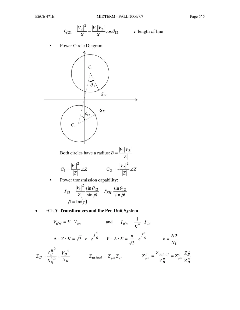Power Circle Diagram C1 C2 S12 -S21 θ12 θ12 Both circles have a radius: Z V V B 2 1 = Z Z V ∠ 2 1 C1 = Z Z V ∠ 2 2 2 - = C � Power transmission capability: l P l Z V P SIL c β θ β θ sin sin sin sin = 12 12 2 1 12 = ( ) γ β = Im • ∗Ch.5: Transformers and the Per-Unit System an a n K V V ′ ′ = and an a n I K I * 1 ′ ′ = 6 3 : jπ n e K Y = ∆ − 6 3 : jπ e n K Y = − ∆ 1 2 N n = N B B B ll B B S V S V Z 2 3 2 = = Φ B pu actual Z Z Z = n B o B o pu n B actual n pu Z Z Z Z Z Z = =