
MATH 202 Useful File Solution Manual, Spring 2011
American University of Beirut · Differential Equations · 736 pages · with solution


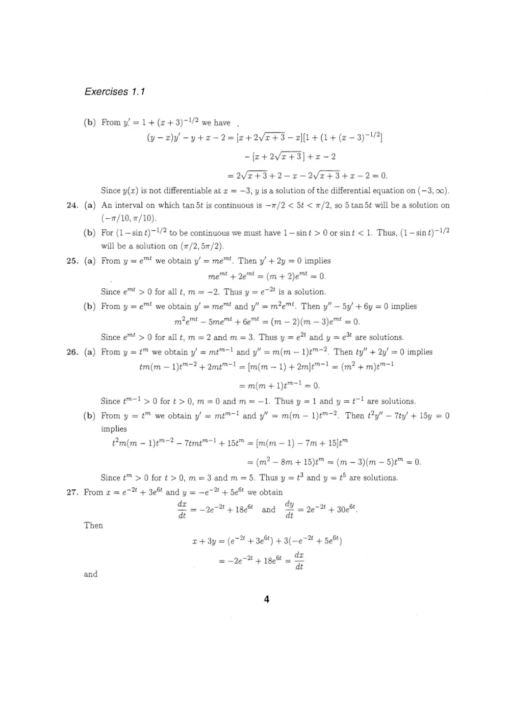
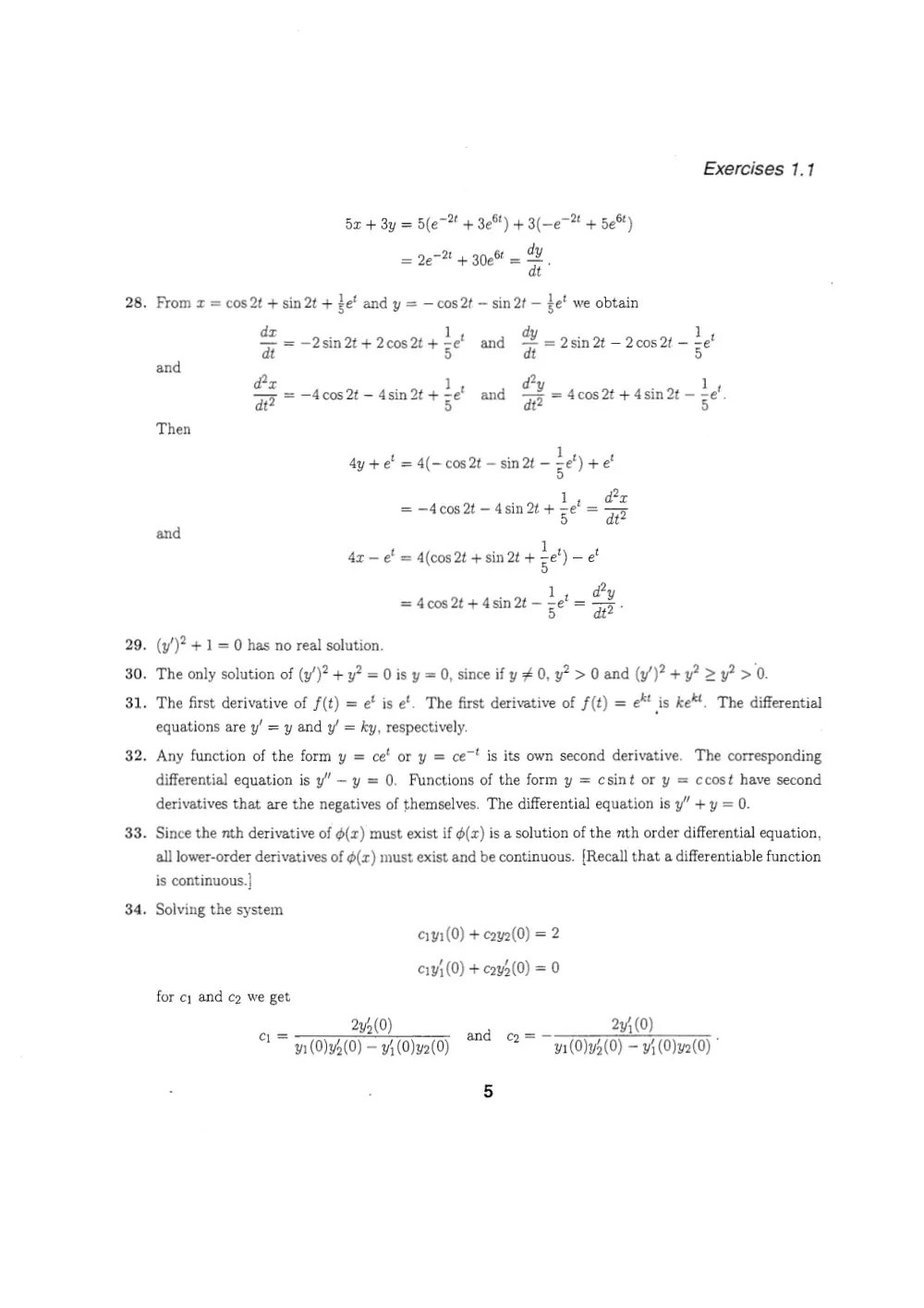
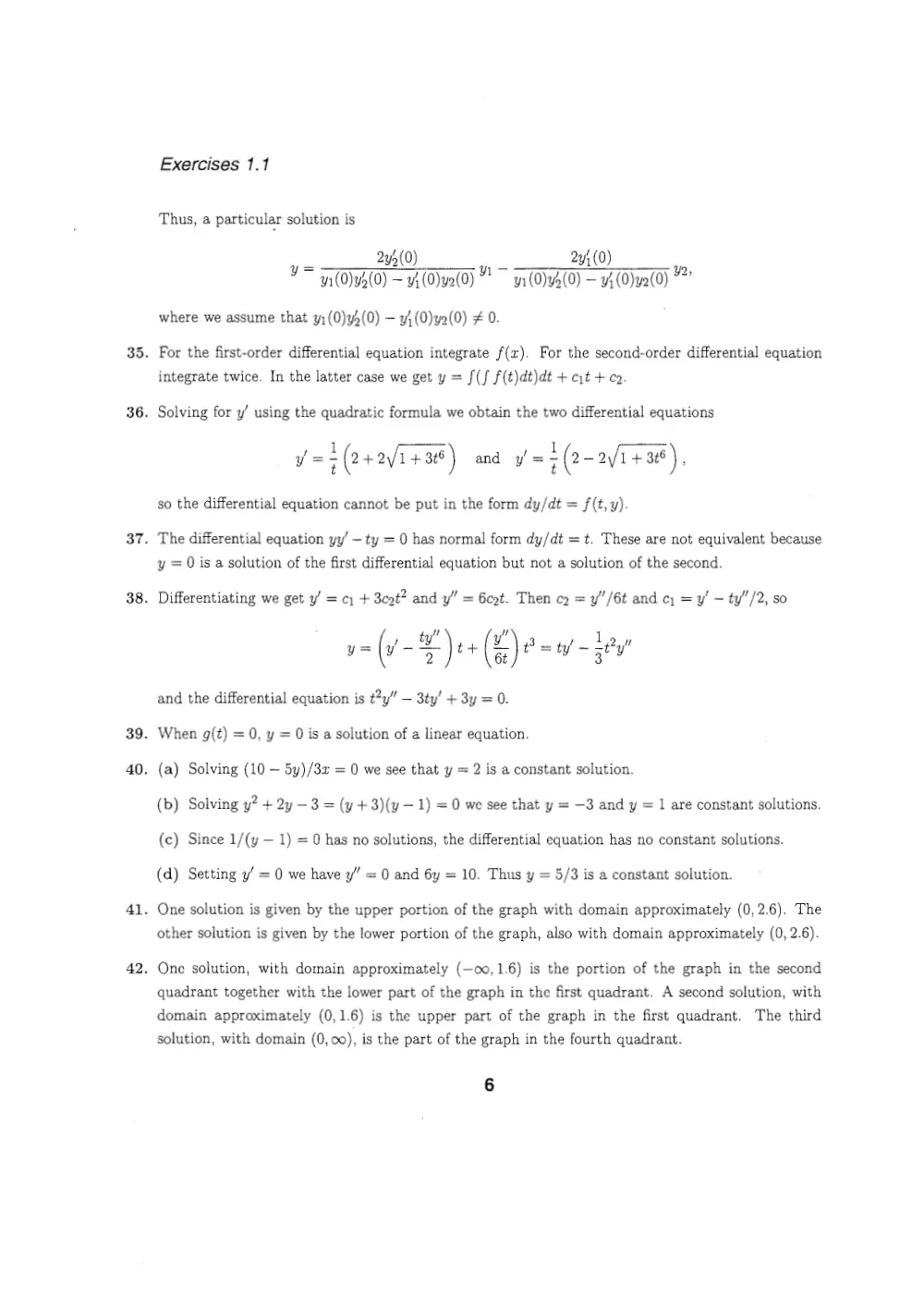
Showing the first 10 of 736 pages. Download the PDF to see all of it.
More MATH 202 files
- Useful File Summary · Spring 2016FileView
- Useful File Summary · Spring 2015FileView
- Useful File Quiz 1 Sample · Spring 2014FileView
- Useful File Elementary Rules of Differentiation · Spring 2011FileView
- Other · Spring 2008FileView
- Useful File · Fall 1998FileView
- Exam Solution to Sample Exam I · Spring 2019Exam · with solutionView
- Syllabus · Spring 2019LabView
Show the text of this file
COMPLETE SOLUTIONS
MANUAL FOR: —
ZILL’S
A FIRST COURSE IN
DIFFERENTIAL
EQUATIONS
WITH MODELING APPLICATIONS
7TH EDITION
AND
ZILL & CULLEN’S
DIFFERENTIAL
EQUATIONS
WITH BOUNDARY-VALUE PROBLEMS
STH EDITION
BROOKS/COLE
S| ete
THOMSON LEARNING
Australia * Canada * Mexico * Singapore + Spain + United Kingdom + United States
Table of Contents
an VW eF WO N
wo on
10
11
12
13
14
15
Appendix I
Appendix II
Introduction to Differential Equations
First-Order Differential Equations
Modeling with First-Order Differential Equations
Higher-Order Differential Equations
Modeling with Higher-Order Differential Equations
Series Solutions of Linear Equations
The Laplace Transform
Systems of Linear First-Order Differential Equations
Numerical Solutions of Ordinary Differential Equations
Plane Autonomous Systems and Stability
Orthogonal Functions and Fourier Series
Partial Differential Equations and Boundary-Value
Problems in Rectangular Coordinates
Boundary-Value Problems in Other Coordinate Systems
Integral Transform Method
Numerical Solutions of Partial Differential Equations
Gamma function
Introduction to Matrices
22
71
104
194
240
308
370
430
458
491
538
616
654
695
717
718
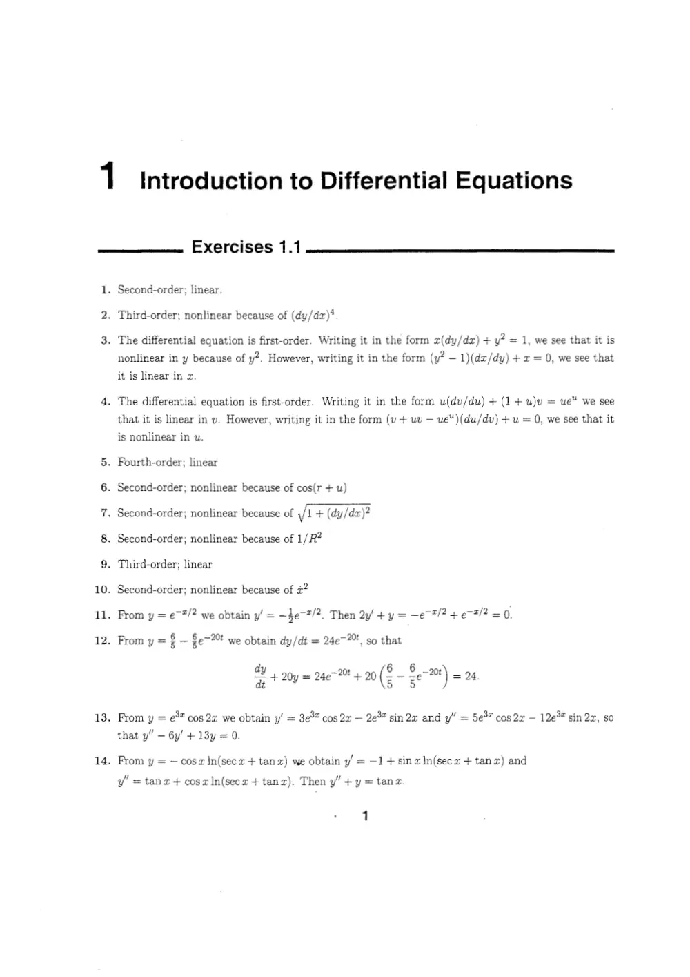
1 Introduction to Differential Equations
10.
11.
12.
13.
14.
Exercises 1.1
. Second-order; linear.
. Third-order; nonlinear because of (dy/dz)*.
. The differential equation is first-order. Writing it in the form 2(dy/dx) + y? = 1, we see that it is
nonlinear in y because of y*. However, writing it in the form (y? — 1)(dz/dy) + 2 = 0, we see that
it is linear in z.
The differential equation is first-order. Writing it in the form u(dv/du) + (1+ u)v = ue” we see
that it is linear in v. However, writing it in the form (v + uv — ue“)(du/dv) + u = 0, we see that it
is nonlinear in u.
. Fourth-order; linear
. Second-order; nonlinear because of cos(r + u)
Second-order; nonlinear because of ,/1 + (dy/dz)?
. Second-order; nonlinear because of 1/R?
. Third-order; linear
Second-order; nonlinear because of <*
From y = e~*/? we obtain y! = —heot/?, Then 2y’+y= —eWt/2 4 eH 2/2 = 0),
From y = £ — $670 we obtain dy/dt = 24e~?°", so that
dy 208 (2 6 “2
=+ = + 20{--= = 24.
pt 20y = 24e 7 + 20 (= — ze
From y = e** cos 2x we obtain y! = 3e%* cos 2x — 2e2* sin 2x and y” = 5e*" cos 2z — 12e3” sin 2z, so
that y” — 6y’ + 13y =0.
From y = — cos zIn(secz + tanz) we obtain y’ = —1 + sinx|n(secz + tanz) and
y! = tanz+coszIn(secr+tanz). Then y” +y = tang.
1
Exercises 1.1
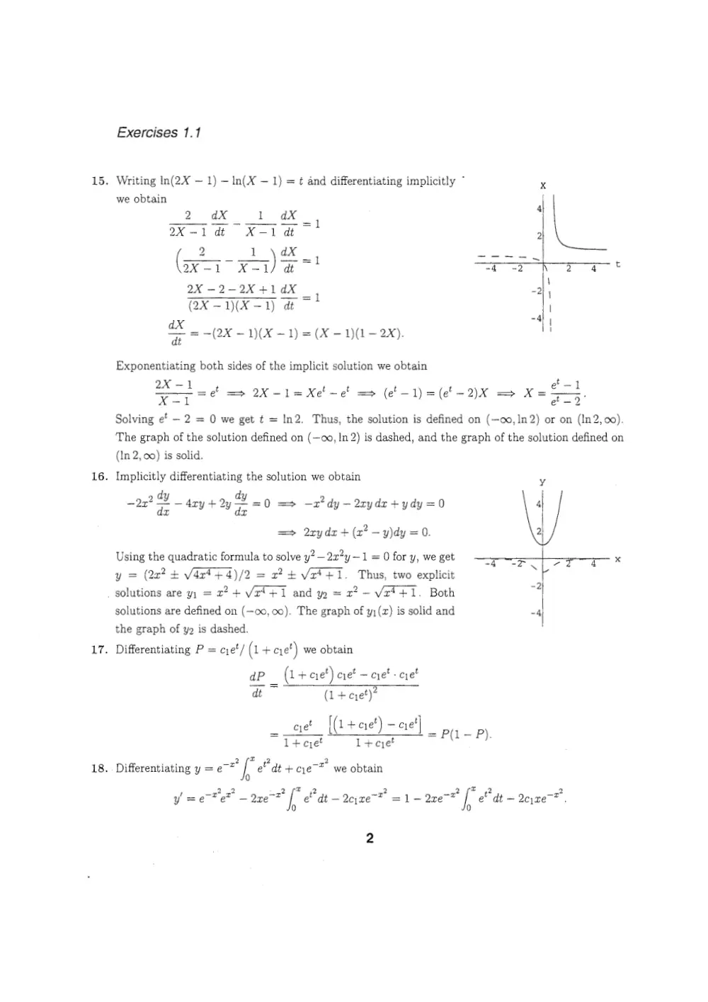
15. Writing In(2X ~ 1) — In(X — 1) = ¢ and differentiating implicitly ~ x
we obtain
2 aX 1 dX _, ‘
2X-1 dt X-1 dt 2
2 1 ) ax _, ~-- +e
Comer “dt —4 2 N24 iF
\
2X -2~-2X+1dX _ -2
(2X —1)(X-1) dt — |
-4
Xx |
af = -(2X ~1(X ~1) =(X 1) - 2X),
Exponentiating both sides of the implicit solution we obtain
xX — fay
2X) Lt <y ox 1 = Xel—e! => (e—1) =(e'-2)X x= S,
X-1 et -2
Solving e’ — 2 = 0 we get t = In2. Thus, the solution is defined on (—oo, 1n2) or on (In2,00).
The graph of the solution defined on (—oo, In 2) is dashed, and the graph of the solution defined on
(In 2, co) is solid.
16. Implicitly differentiating the solution we obtain
y
d d:
— 22? — day + 2y 4 =0 = -2° dy -2cydz+ydy =0 4
=> 2xydz + (x? — y)dy = 0. 2
Using the quadratic formula to solve y?—2x2y—1 = 0 for y, we get
y = (22? + Var? +4)/2 = 2? + Vet +1. Thus, two explicit
_ solutions are yy = 22 + V2t +71 and y = x? — Vz? +1. Both °
solutions are defined on (—oo, 00). The graph of y;(z) is solid and ~4
the graph of yg is dashed.
17. Differentiating P = cye’/ (a + ce’) we obtain
dP (1 + ce’) ce’ — cyet - cyet
dt (1 +cyet)”
cyet [(1 + ce’) - ce]
~ 1+cyet 1l+cyet
= P(1- P).
2 fe 42 2
18. Differentiating y =e I eb dt+cje-* we obtain
2
/ —2" 2 a2? [* e ~2? ~2? = 2
y =e *e* —2zre f eat —2c126 =1-2ze » ° dt — 2c\xe~” .
2
19.
20.
21.
22.
23.
Exercises 1.1
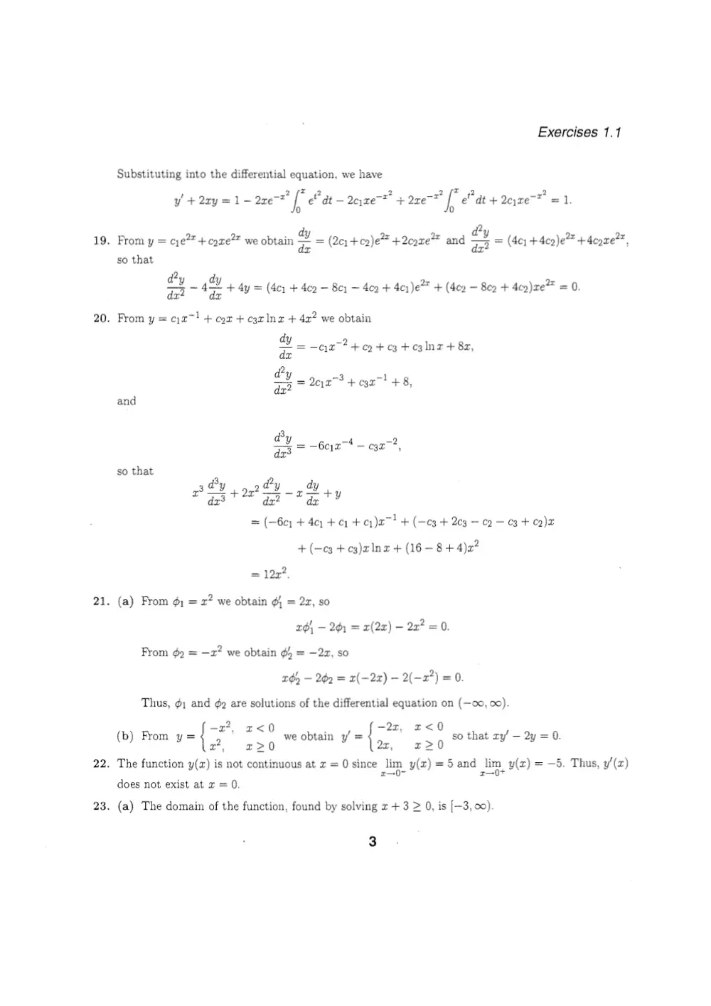
Substituting into the differential equation, we have
© 2st 42 2
y +22y=1- aze~*" [ edt — 2eyne-?" + 2re7* | edt +2cre7*_ = 1.
0
= ert Qe . Qa Qe dy — (Ap Qe Qe
From y = c)e** + coze** we obtain a (2c) +c2)e** +2core~* and ie (4c1 +4c2)e** +4coxe™*,
so that
dy dy Qe on
aaa 7 45m + 4y = (41 + 42 — 8¢1 — 4c + 4c )e* + (4c2 — 8c2 + 4c9)re* = 0.
dz dx
From y = cjz7! + cox + c3z nz + 42? we obtain
d
YX -qa? +co+c3 +c3lnzr + 8g,
dz
a
a = 2e,273 + c3z7} +8,
and
fia
pad =-6cjr * — cx”,
so that , ,
d°y d*y dy
3 2 q
<f 429? Fg Sy
Pa a a TY
= (—6c + 4c) + cy +c )a7! + (—c3 + 203 — co — 03 + co) 0
+(—c3 +c3)elnz+(16-8+ 4)a?
= 1227.
(a) From ¢) = 2? we obtain ¢} = 2z, so
1 — 2g) = x(2x) — 22? = 0.
From ¢) = —2? we obtain $4 = —2z, so
xb — 27 = 2(—2x) — 2(—2?) = 0.
Thus, ¢; and @» are solutions of the differential equation on (—00, 00).
2
-2", 2£<0 -2r, £<0
b) Fr - ’ " in y= , that ry’ — 2y = 0.
(b) From y {2 2>0 we obtain y/ { 2>0 so that ry’ — 2y
The function y(x) is not continuous at x = 0 since lim y(x) = 5 and lim, y(xz) = —5. Thus, y/(x)
2-07 rr
does not exist at x = 0.
(a) The domain of the function, found by solving z + 3 > 0, is [—3, 00).
3
24.
25.
26.
27.
Exercises 1.1
(b) From y!=1+(z+3)7'/? we have .
(y—2)y -yt+2-2= [2+2Vr43—a)[14 (14 (x - 3)
-[c+2Vr+3]+2-2
=2/Vr+34+2-2-2Vr4+34+2-2=0.
Since y(zx) is not differentiable at x = —3, y is a solution of the differential equation on (—3, 00).
(a) An interval on which tan 5t is continuous is —1/2 < 5t < m/2, so 5 tan 5¢ will be a solution on
(—1/10, 7/10).
(b) For (1—sint)~!/? to be continuous we must have 1—sint > 0 or sint < 1. Thus, (1—sint)7!/?
will be a solution on (7/2, 57/2).
(a) From y = e™ we obtain y’ = me™. Then y’ + 2y = 0 implies
me™ +4 2 = (m+2)e™ = 0.
~2 is a solution.
Since e™ > 0 for all t, m = —2. Thus y =e
(b) From y = e™ we obtain y! = me™ and y” = m2e™. Then y” — 5y! + 6y = 0 implies
me™ — 5me™ + 6e™ = (m — 2)(m—3)e™ =0.
3t are solutions.
Since e > 0 for all t, m= 2 and m=3. Thus y = e* andy =e
(a) From y = t™ we obtain y’ = mt™~! and y” = m(m — 1)t™~?. Then ty” + 2y’ = 0 implies
tm(m —1)t™-? + 2met™! = [m(m — 1) + 2m]t™") = (Mm? + m)t™!
= m(m+1)t™-! =0.
Since t”-! > 0 fort > 0, m=0 and m= —1. Thus y = 1 and y = ¢7! are solutions.
(b) From y = t” we obtain y! = mt™~! and y” = m(m — 1)t™-?. Then é?y” — 7ty! + l5y = 0
implies
t?m(m — 1)t™-? — Teme! + 15t™ = [m(m — 1) — 7m + 15]t™
= (m? — 8m + 15)t™ = (m — 3)(m —5)t™ =0.
Since t” > 0 for t > 0, m=3 and m=5. Thus y = # and y = @° are solutions.
From x = e7 + 3e% and y = —e~* + 5e% we obtain
dy
dz ~2t 6t ! ~2t 6t
— =~ _2 =
a 2e~“* + 18e" and at 2e~~ + 30e"".
Then
x +3y = (e~* + 3e%) + 3(-e7* + 528)
dz
= —2e7! 6t
2e~™ + 18e Zi
and
28.
29.
30.
31.
32.
33.
34.
Exercises 1.1
5a + 3y = 5(e7*! + 3e%) + 3(-e7-% + 5e%)
d
= 27% + 30e% = 2,
dt
From x = cos 2t + sin 2t + de’ and y = —cos2t — sin 2t — fe! we obtain
dz 1 d . 1
a —2sin 2t + 2cos 2t + ze and ra 2sin 2t — 2cos 2t — ze
and 5 5
d-x 1 d* . 1
mo —4cos 2t — 4sin 2t+ ze and a = 4cos 2t + 4sin 2t — ze
Then
t_ _¢; li t
4y +e = 4(—cos 2t — sin 2t — 5e )+e
1 a
= —4cos 2t — 4sin 2t + ze =
and ;
4x —e' = 4(cos2t +sin 2¢ + ze) -eé
1 d?
= 4cos 2t + 4sin 2t — ze = ae
(y')? + 1 =0 has no real solution.
The only solution of (y’)? + y? = 0 is y = 0, since if y #0, y2 > O and (y')? +y2 >y? >0.
The first derivative of f(t) = et is et. The first derivative of f(t) = e* is ke. The differential
equations are y' = y and y’ = ky, respectively.
* is its own second derivative. The corresponding
Any function of the form y = ce’ or y = ce7
differential equation is y’ — y = 0. Functions of the form y = csint or y = ccost have second
derivatives that are the negatives of themselves. The differential equation is y” + y = 0.
Since the nth derivative of 6(x) must exist if 6(x) is a solution of the nth order differential equation,
all lower-order derivatives of ¢(x) must exist and be continuous. {Recall that a differentiable function
is continuous.}
Solving the system
e1yi(0) + coyo(0) = 2
ery} (0) + coy9(0) =
for cy and cp we get
_ 2uh(0)
wi(0)u8(0) — vj(0)u2(0)
2y;,(0)
and = ~FOwhl0) — v4 (Ou0(0)
c]
35.
36.
37.
38.
39.
40.
41.
42.
Exercises 1.1
Thus, a particular solution is
_ 2yh(0) 7 2y4 (0) b
nil0yvh(0) — vi(Oyya0) 2 ~ yr (Oy (0) — viO)uaC0)
where we assume that yi (0)y$(0) — y}(0)ye(0) 4 0.
For the first-order differential equation integrate f(x). For the second-order differential equation
integrate twice. In the latter case we get y = f(f f(t)dt)dt + cit +c.
Solving for y’ using the quadratic formula we obtain the two differential equations
v => (2+2yi+38) and y => (2-2V1+38),
so the differential equation cannot be put in the form dy/dt = f(t, y).
The differential equation yy’ — ty = 0 has normal form dy/dt = t. These are not equivalent because
y = 0 is a solution of the first differential equation but not a solution of the second.
Differentiating we get y’ = c) + 3cot” and y” = 6cgt. Then cp = y"/6t and c, = y’ — ty"/2, so
, ty’ y" 3 J 1 2,
= -—> —jt=ty-->
y (v tle y aby
and the differential equation is t?y” — 3ty’ + 3y = 0.
When g(t) = 0, y = 0 is a solution of a linear equation.
(a) Solving (10 — 5y)/3x = 0 we see that y = 2 is a constant solution.
(b) Solving y* + 2y —3 = (y+3)(y—1) =0 we see that y = —3 and y = 1 are constant solutions.
(c) Since 1/(y — 1) = 0 has no solutions, the differential equation has no constant solutions.
(d) Setting y’ = 0 we have y” = 0 and 6y = 10. Thus y = 5/3 is a constant solution.
One solution is given by the upper portion of the graph with domain approximately (0, 2.6). The
other solution is given by the lower portion of the graph, also with domain approximately (0, 2.6).
One solution, with domain approximately (—oo, 1.6) is the portion of the graph in the second
quadrant together with the lower part of the graph in the first quadrant. A second solution, with
domain approximately (0,1.6) is the upper part of the graph in the first quadrant. The third
solution, with domain (0, 00), is the part of the graph in the fourth quadrant.
6