MATH 202 Useful File Summary, Spring 2016

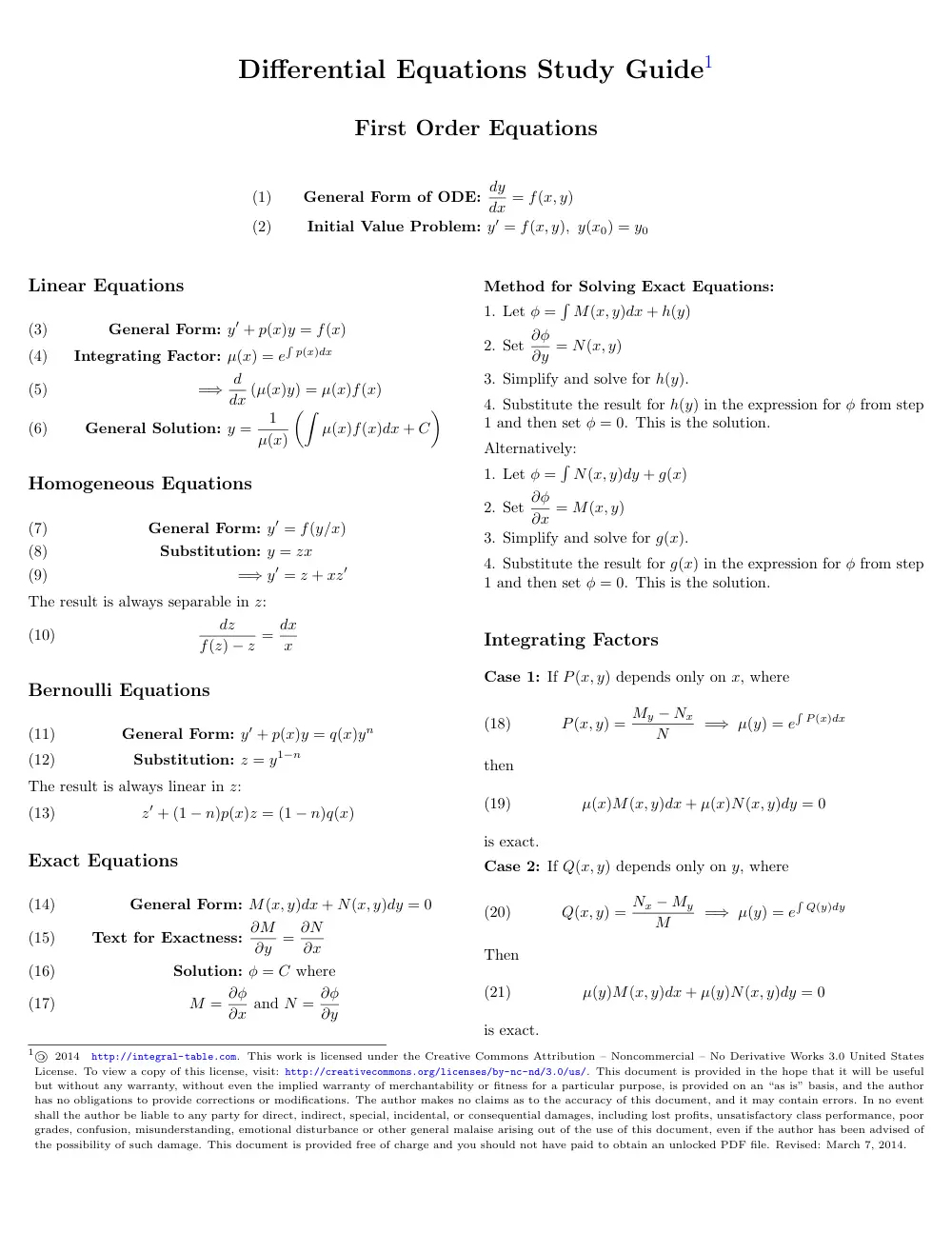
Differential Equations Study Guide1 First Order Equations General Form of ODE: dy dx = f(x, y) (1) Initial Value Problem: y′ = f(x, y), y(x0) = y0 (2) Linear Equations General Form: y′ + p(x)y = f(x) (3) Integrating Factor: µ(x) = e � p(x)dx (4) =⇒ d dx (µ(x)y) = µ(x)f(x) (5) General Solution: y = 1 µ(x) �� µ(x)f(x)dx + C � (6) Homogeneous Equations General Form: y′ = f(y/x) (7) Substitution: y = zx (8) =⇒ y′ = z + xz′ (9) The result is always separable in z: (10) dz f(z) − z = dx x Bernoulli Equations General Form: y′ + p(x)y = q(x)yn (11) Substitution: z = y1−n (12) The result is always linear in z: (13) z′ + (1 − n)p(x)z = (1 − n)q(x) Exact Equations General Form: M(x, y)dx + N(x, y)dy = 0 (14) Text for Exactness: ∂M ∂y = ∂N ∂x (15) Solution: φ = C where (16) M = ∂φ ∂x and N = ∂φ ∂y (17) Method for Solving Exact Equations: 1. Let φ = � M(x, y)dx + h(y) 2. Set ∂φ ∂y = N(x, y) 3. Simplify and solve for h(y). 4. Substitute the result for h(y) in the expression for φ from step 1 and then set φ = 0. This is the solution. Alternatively: 1. Let φ = � N(x, y)dy + g(x) 2. Set ∂φ ∂x = M(x, y) 3. Simplify and solve for g(x). 4. Substitute the result for g(x) in the expression for φ from step 1 and then set φ = 0. This is the solution. Integrating Factors Case 1: If P(x, y) depends only on x, where (18) P(x, y) = My − Nx N =⇒ µ(y) = e � P (x)dx then (19) µ(x)M(x, y)dx + µ(x)N(x, y)dy = 0 is exact. Case 2: If Q(x, y) depends only on y, where (20) Q(x, y) = Nx − My M =⇒ µ(y) = e � Q(y)dy Then (21) µ(y)M(x, y)dx + µ(y)N(x, y)dy = 0 is exact. 1� 2014 http://integral-table.com. This work is licensed under the Creative Commons Attribution – Noncommercial – No Derivative Works 3.0 United States License. To view a copy of this license, visit: http://creativecommons.org/licenses/by-nc-nd/3.0/us/. This document is provided in the hope that it will be useful but without any warranty, without even the implied warranty of merchantability or fitness for a particular purpose, is provided on an “as is” basis, and the author has no obligations to provide corrections or modifications. The author makes no claims as to the accuracy of this document, and it may contain errors. In no event shall the author be liable to any party for direct, indirect, special, incidental, or consequential damages, including lost profits, unsatisfactory class performance, poor grades, confusion, misunderstanding, emotional disturbance or other general malaise arising out of the use of this document, even if the author has been advised of the possibility of such damage. This document is provided free of charge and you should not have paid to obtain an unlocked PDF file. Revised: March 7, 2014. 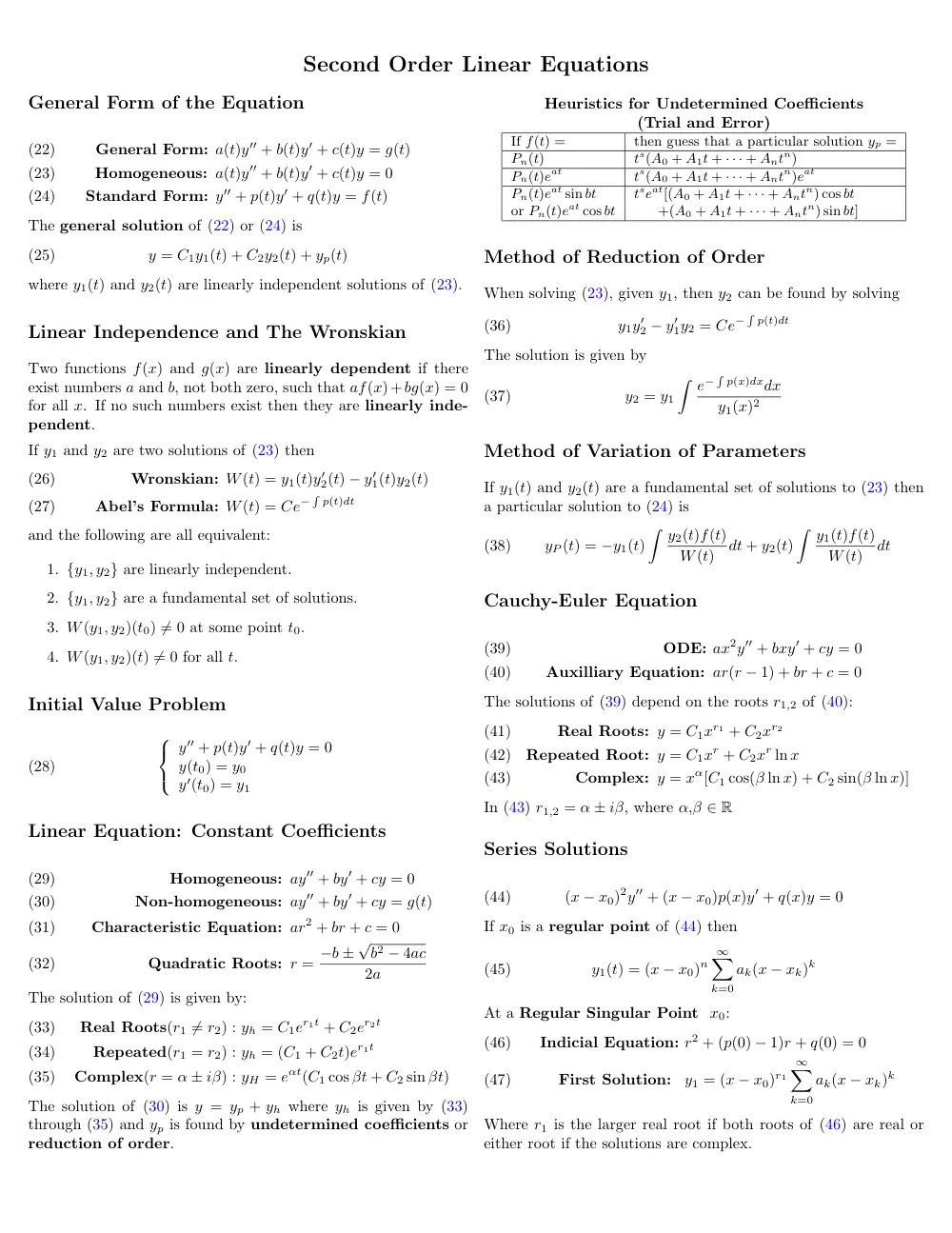Second Order Linear Equations General Form of the Equation General Form: a(t)y′′ + b(t)y′ + c(t)y = g(t) (22) Homogeneous: a(t)y′′ + b(t)y′ + c(t)y = 0 (23) Standard Form: y′′ + p(t)y′ + q(t)y = f(t) (24) The general solution of (22) or (24) is (25) y = C1y1(t) + C2y2(t) + yp(t) where y1(t) and y2(t) are linearly independent solutions of (23). Linear Independence and The Wronskian Two functions f(x) and g(x) are linearly dependent if there exist numbers a and b, not both zero, such that af(x)+bg(x) = 0 for all x. If no such numbers exist then they are linearly inde- pendent. If y1 and y2 are two solutions of (23) then Wronskian: W(t) = y1(t)y′ 2(t) − y′ 1(t)y2(t) (26) Abel’s Formula: W(t) = Ce− � p(t)dt (27) and the following are all equivalent: 1. {y1, y2} are linearly independent. 2. {y1, y2} are a fundamental set of solutions. 3. W(y1, y2)(t0) ̸= 0 at some point t0. 4. W(y1, y2)(t) ̸= 0 for all t. Initial Value Problem (28)    y′′ + p(t)y′ + q(t)y = 0 y(t0) = y0 y′(t0) = y1 Linear Equation: Constant Coefficients Homogeneous: ay′′ + by′ + cy = 0 (29) Non-homogeneous: ay′′ + by′ + cy = g(t) (30) Characteristic Equation: ar2 + br + c = 0 (31) Quadratic Roots: r = −b ± √ b2 − 4ac 2a (32) The solution of (29) is given by: Real Roots(r1 ̸= r2) : yh = C1er1t + C2er2t (33) Repeated(r1 = r2) : yh = (C1 + C2t)er1t (34) Complex(r = α ± iβ) : yH = eαt(C1 cos βt + C2 sin βt) (35) The solution of (30) is y = yp + yh where yh is given by (33) through (35) and yp is found by undetermined coefficients or reduction of order. Heuristics for Undetermined Coefficients (Trial and Error) If f(t) = then guess that a particular solution yp = Pn(t) ts(A0 + A1t + · · · + Antn) Pn(t)eat ts(A0 + A1t + · · · + Antn)eat Pn(t)eat sin bt tseat[(A0 + A1t + · · · + Antn) cos bt or Pn(t)eat cos bt +(A0 + A1t + · · · + Antn) sin bt] Method of Reduction of Order When solving (23), given y1, then y2 can be found by solving (36) y1y′ 2 − y′ 1y2 = Ce− � p(t)dt The solution is given by (37) y2 = y1 � e− � p(x)dxdx y1(x)2 Method of Variation of Parameters If y1(t) and y2(t) are a fundamental set of solutions to (23) then a particular solution to (24) is (38) yP (t) = −y1(t) � y2(t)f(t) W(t) dt + y2(t) � y1(t)f(t) W(t) dt Cauchy-Euler Equation ODE: ax2y′′ + bxy′ + cy = 0 (39) Auxilliary Equation: ar(r − 1) + br + c = 0 (40) The solutions of (39) depend on the roots r1,2 of (40): Real Roots: y = C1xr1 + C2xr2 (41) Repeated Root: y = C1xr + C2xr ln x (42) Complex: y = xα[C1 cos(β ln x) + C2 sin(β ln x)] (43) In (43) r1,2 = α ± iβ, where α,β ∈ R Series Solutions (44) (x − x0)2y′′ + (x − x0)p(x)y′ + q(x)y = 0 If x0 is a regular point of (44) then (45) y1(t) = (x − x0)n ∞ � k=0 ak(x − xk)k At a Regular Singular Point x0: Indicial Equation: r2 + (p(0) − 1)r + q(0) = 0 (46) First Solution: y1 = (x − x0)r1 ∞ � k=0 ak(x − xk)k (47) Where r1 is the larger real root if both roots of (46) are real or either root if the solutions are complex.