MECH 314 Notes 8, Spring 2014

MECH 314 Introduction to Fluid Mechanics February 19, 2009 American University of Beirut, Spring 2009 Handout # 4 Integral Relations for a Control Volume 1. (Lecture 1) Control Volume vs System System: a collection of matter of fixed identity. Control Volume: is a volume fixed in the coordinated frame of reference and is bounded a control surface. 2. (Lecture 1) Fundamentals physical laws for a system in primitive form We are often interested in the rate of change of the amount of a certain physical property contained in a system of volume V . The physical property could be mass, momentum, energy, moment of momentum, entropy etc. The amount of physical property contained in V may be expressed as B ≡ � V bρ dV so that the rate of change is DB Dt . The fundamental physical laws governing the rate of change of B is DB Dt = Φ. The table below presents the physical laws of conservation of mass, momentum and energy expressed in the form dB dt = Φ. Conservation Law b B Φ mass 1 total mass: � V ρ dV 0 linear momentum u total momentum: � V ρu dV � F angular momentum r × u total momentum: � V ρ(r × u) dV � MO energy e + |u|2 2 + U total energy: � V ρ � e + |u|2 2 + U � dV � δ ˙q − � δ ˙w where ρ is density, u is velocity vector, r is position vector, e is sepcific internal energy, U is potential energy, � F is the sum of all the forces (surface and body) acting on the control volume, � MO is the sum of all the moments about point O applied to the control volume, � δ ˙q is the sum of heat gained by the comtrol volume, and � δ ˙w is the sum of work done by the control volume (shaft, pressure, viscous stresses). 3. The need for a control volume approach and the Reynolds Transport Theorem In fluid mechanics, a system undergoes changes in its shape ans volume. It could experience stretching, twisting, expansion etc. It is therefore difficult to predict V in a Lagrangian sense. It is more convenient to apply the laws of physics for a control volume since it is a fixed volume. In order to apply the above physical laws for a control volume, we need to express the rate of change of the total quantity B in terms of rate of change inside the control volume and fluxes crossing the control surface. In other words: D Dt � V bρ dV ?→ (?)C.V. 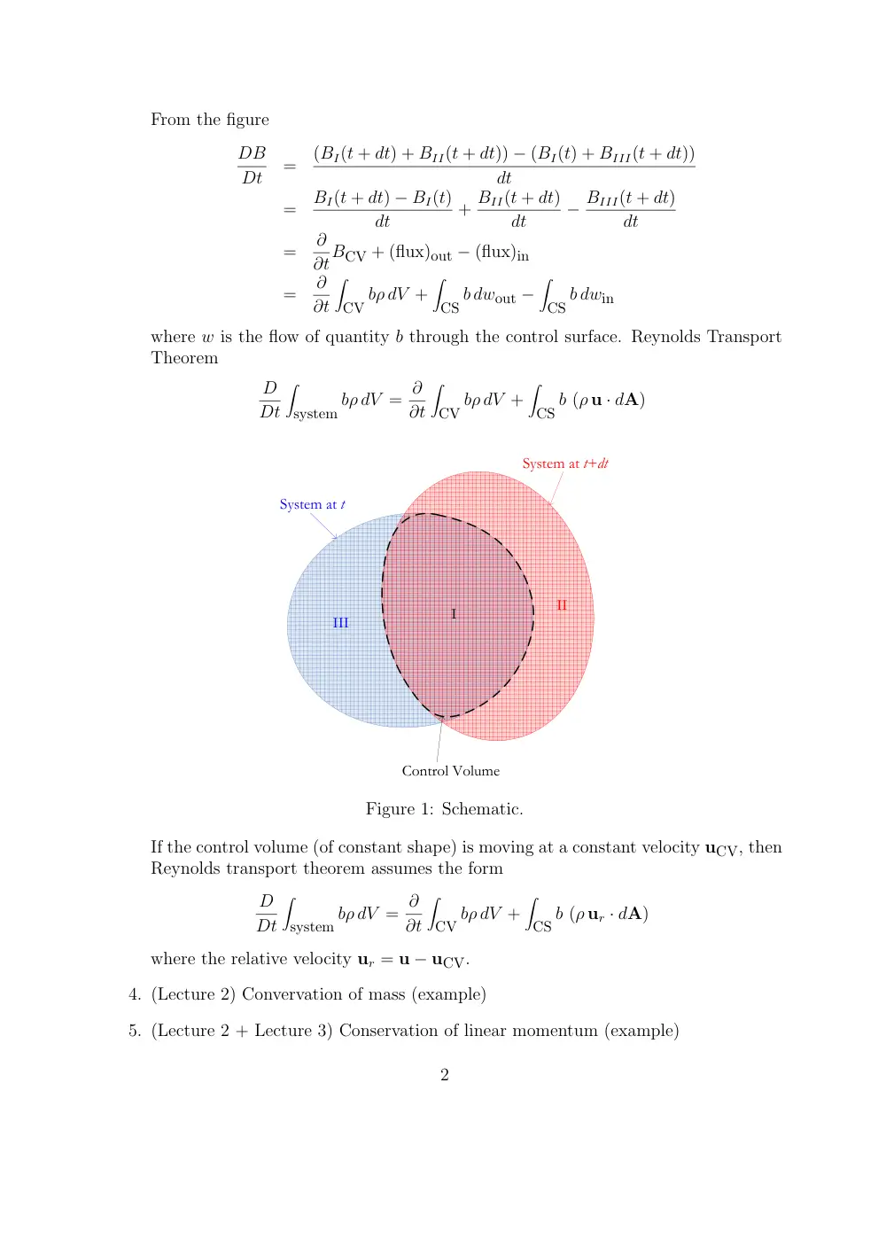1 From the figure DB Dt = (BI(t + dt) + BII(t + dt)) − (BI(t) + BIII(t + dt)) dt = BI(t + dt) − BI(t) dt + BII(t + dt) dt − BIII(t + dt) dt = ∂ ∂tBCV + (flux)out − (flux)in = ∂ ∂t � CV bρ dV + � CS b dwout − � CS b dwin where w is the flow of quantity b through the control surface. Reynolds Transport Theorem D Dt � system bρ dV = ∂ ∂t � CV bρ dV + � CS b (ρ u · dA) System at t System at t+dt Control Volume III II I Figure 1: Schematic. If the control volume (of constant shape) is moving at a constant velocity uCV, then Reynolds transport theorem assumes the form D Dt � system bρ dV = ∂ ∂t � CV bρ dV + � CS b (ρ ur · dA) where the relative velocity ur = u − uCV. 4. (Lecture 2) Convervation of mass (example) 5. (Lecture 2 + Lecture 3) Conservation of linear momentum (example) 2 6. (Lecture 3) Conservation of angular momentum (example) 7. (Lecture 4) Conservation of energy (example) Read: White Sections 3.1-3.6 3