MECH 314 Notes 9, Spring 2014

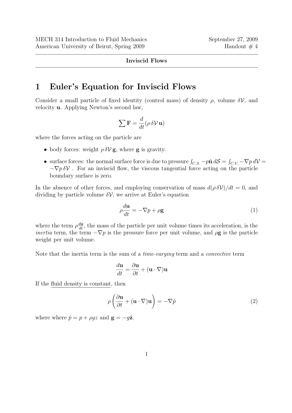
MECH 314 Introduction to Fluid Mechanics September 27, 2009 American University of Beirut, Spring 2009 Handout # 4 Inviscid Flows 1 Euler’s Equation for Inviscid Flows Consider a small particle of fixed identity (control mass) of density ρ, volume δV, and velocity u. Applying Newton’s second law, � F = d dt(ρ δV u) where the forces acting on the particle are • body forces: weight ρ δV g, where g is gravity. • surface forces: the normal surface force is due to pressure � C.S. −pˆn dS = � C.V. −∇p dV = −∇p δV . For an inviscid flow, the viscous tangential force acting on the particle boundary surface is zero. In the absence of other forces, and employing conservation of mass d(ρ δV)/dt = 0, and dividing by particle volume δV, we arrive at Euler’s equation ρdu dt = −∇p + ρg (1) where the term ρ du dt , the mass of the particle per unit volume times its acceleration, is the inertia term, the term −∇p is the pressure force per unit volume, and ρg is the particle weight per unit volume. Note that the inertia term is the sum of a time-varying term and a convective term du dt = ∂u ∂t + (u · ∇)u If the fluid density is constant, then ρ �∂u ∂t + (u · ∇)u � = −∇ˆp (2) where where ˆp = p + ρgz and g = −gˆz. 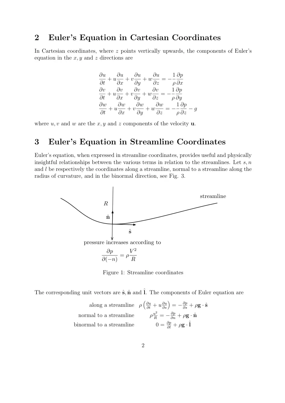1 2 Euler’s Equation in Cartesian Coordinates In Cartesian coordinates, where z points vertically upwards, the components of Euler’s equation in the x, y and z directions are ∂u ∂t + u∂u ∂x + v∂u ∂y + w∂u ∂z = −1 ρ ∂p ∂x ∂v ∂t + u∂v ∂x + v∂v ∂y + w∂v ∂z = −1 ρ ∂p ∂y ∂w ∂t + u∂w ∂x + v∂w ∂y + w∂w ∂z = −1 ρ ∂p ∂z − g where u, v and w are the x, y and z components of the velocity u. 3 Euler’s Equation in Streamline Coordinates Euler’s equation, when expressed in streamline coordinates, provides useful and physically insightful relationships between the various terms in relation to the streamlines. Let s, n and l be respectively the coordinates along a streamline, normal to a streamline along the radius of curvature, and in the binormal direction, see Fig. 3. R ˆs ˆn streamline pressure increases according to ∂p ∂(−n) = ρV 2 R Figure 1: Streamline coordinates The corresponding unit vectors are ˆs, ˆn and ˆl. 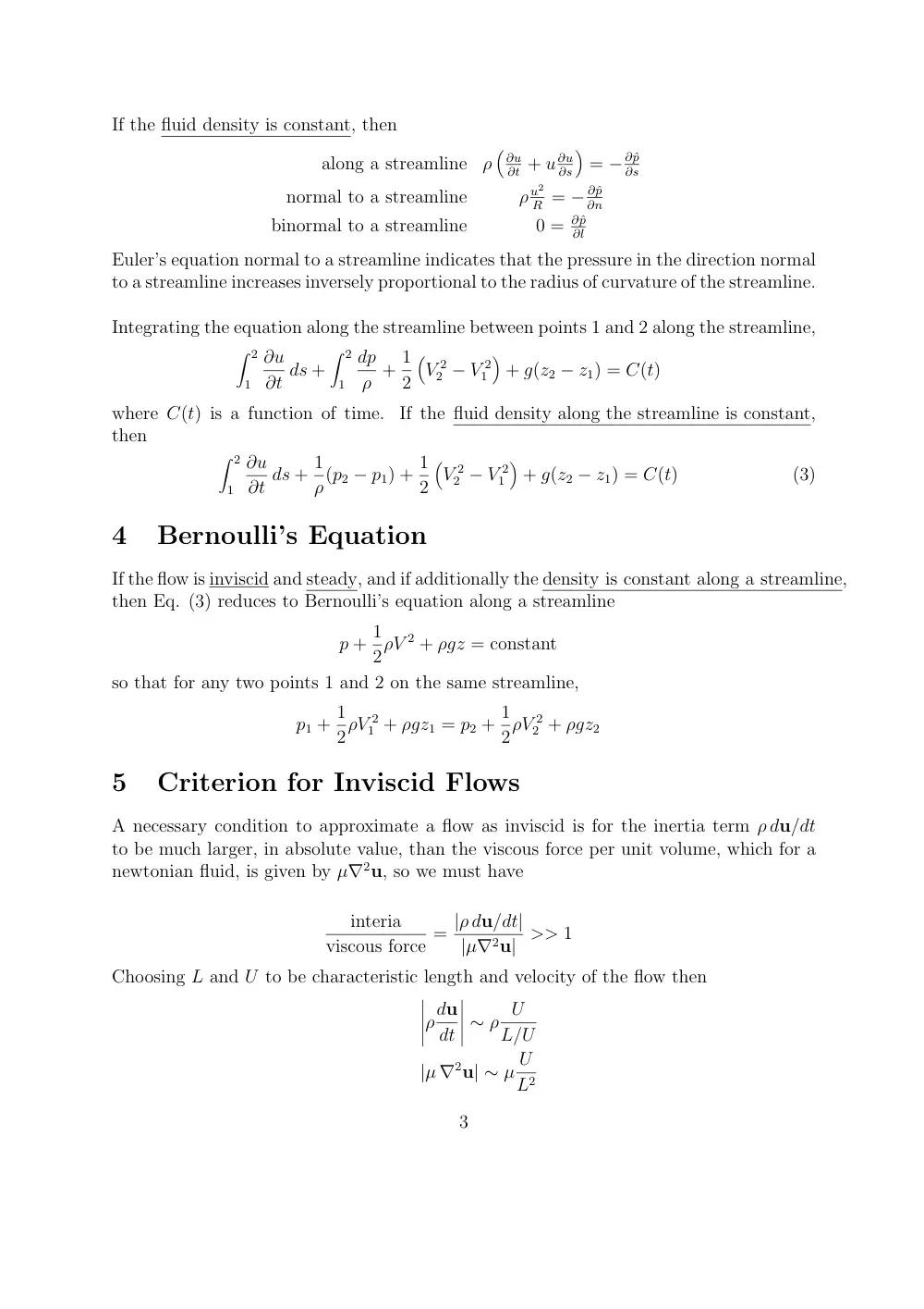The components of Euler equation are along a streamline ρ � ∂u ∂t + u ∂u ∂s � = −∂p ∂s + ρg · ˆs normal to a streamline ρ u2 R = − ∂p ∂n + ρg · ˆn binormal to a streamline 0 = ∂p ∂l + ρg ·ˆl 2 If the fluid density is constant, then along a streamline ρ � ∂u ∂t + u ∂u ∂s � = −∂ˆp ∂s normal to a streamline ρ u2 R = − ∂ˆp ∂n binormal to a streamline 0 = ∂ˆp ∂l Euler’s equation normal to a streamline indicates that the pressure in the direction normal to a streamline increases inversely proportional to the radius of curvature of the streamline. Integrating the equation along the streamline between points 1 and 2 along the streamline, � 2 1 ∂u ∂t ds + � 2 1 dp ρ + 1 2 � V 2 2 − V 2 1 � + g(z2 − z1) = C(t) where C(t) is a function of time. If the fluid density along the streamline is constant, then � 2 1 ∂u ∂t ds + 1 ρ(p2 − p1) + 1 2 � V 2 2 − V 2 1 � + g(z2 − z1) = C(t) (3) 4 Bernoulli’s Equation If the flow is inviscid and steady, and if additionally the density is constant along a streamline, then Eq. (3) reduces to Bernoulli’s equation along a streamline p + 1 2ρV 2 + ρgz = constant so that for any two points 1 and 2 on the same streamline, p1 + 1 2ρV 2 1 + ρgz1 = p2 + 1 2ρV 2 2 + ρgz2 5 Criterion for Inviscid Flows A necessary condition to approximate a flow as inviscid is for the inertia term ρ du/dt to be much larger, in absolute value, than the viscous force per unit volume, which for a newtonian fluid, is given by µ∇2u, so we must have interia viscous force = |ρ du/dt| |µ∇2u| >> 1 Choosing L and U to be characteristic length and velocity of the flow then �����ρdu dt ����� ∼ ρ U L/U |µ ∇2u| ∼ µ U L2 3 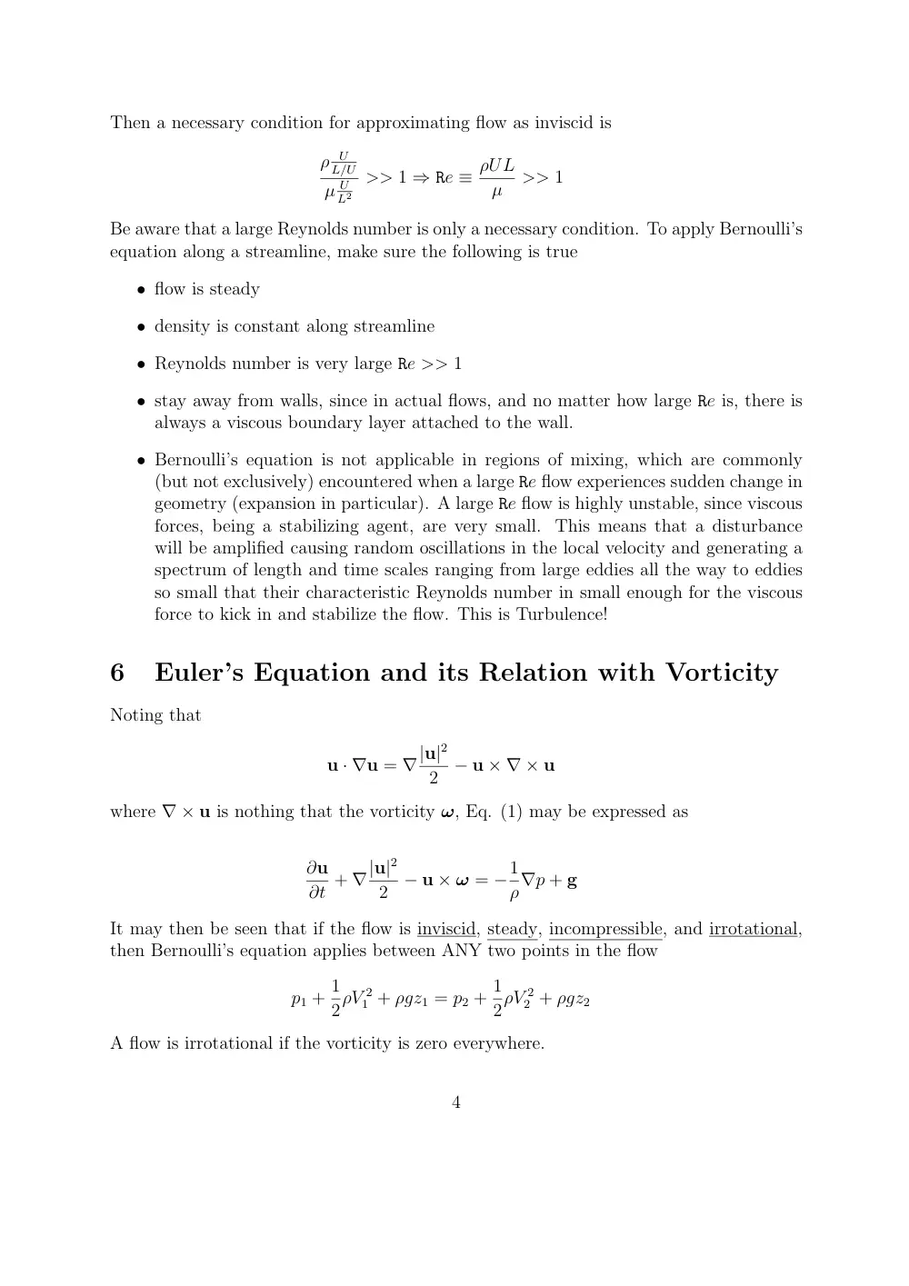Then a necessary condition for approximating flow as inviscid is ρ U L/U µ U L2 >> 1 ⇒ Re ≡ ρUL µ >> 1 Be aware that a large Reynolds number is only a necessary condition. To apply Bernoulli’s equation along a streamline, make sure the following is true • flow is steady • density is constant along streamline • Reynolds number is very large Re >> 1 • stay away from walls, since in actual flows, and no matter how large Re is, there is always a viscous boundary layer attached to the wall. • Bernoulli’s equation is not applicable in regions of mixing, which are commonly (but not exclusively) encountered when a large Re flow experiences sudden change in geometry (expansion in particular). A large Re flow is highly unstable, since viscous forces, being a stabilizing agent, are very small. This means that a disturbance will be amplified causing random oscillations in the local velocity and generating a spectrum of length and time scales ranging from large eddies all the way to eddies so small that their characteristic Reynolds number in small enough for the viscous force to kick in and stabilize the flow. This is Turbulence! 6 Euler’s Equation and its Relation with Vorticity Noting that u · ∇u = ∇|u|2 2 − u × ∇ × u where ∇ × u is nothing that the vorticity ω, Eq. (1) may be expressed as ∂u ∂t + ∇|u|2 2 − u × ω = −1 ρ∇p + g It may then be seen that if the flow is inviscid, steady, incompressible, and irrotational, then Bernoulli’s equation applies between ANY two points in the flow p1 + 1 2ρV 2 1 + ρgz1 = p2 + 1 2ρV 2 2 + ρgz2 A flow is irrotational if the vorticity is zero everywhere. 4