PHYS 212 Notes Quantum Mechanics, Spring 2017

Quantum Mechanics J.K. October 7, 1900 1 Introduction Before the beginning Quantum Mechanics, there were many phenomena that needed explanation as the theories of the time failed to predict them, or to explain them. Blackbody Radiation: A blackbody refers to an opaque object that emits thermal radiation. The ultraviolet catastrophe was the prediction of late 19th century/early 20th century classical physics that an ideal black body at thermal equilibrium will emit radiation in all frequency ranges, emitting more energy as the frequency increases. By calculating the total amount of radiated energy a blackbody would release an infinite amount of energy, contradicting the principles of conservation of energy. Planck solved this issue using statistical mechanics on the 7th of October 1900. He postulated that electromagnetic radiation can only be emitted or absorbed in discrete packets, called quanta, such that EQuanta = ¯hw = hf where h is Planck’s constant ( h = 6.6260755x10−34Js ), f is the frequency of light, w is the angular frequency of light, and ¯h = h 2 . Another issue was the photoelectric effect, the emission of electrons or other free carriers when light is shone onto a material. In 1905, Albert Einstein used Planck’s postulate to explain this phenomena. A photon above a threshold frequency has the required energy to eject a single electron, creating the observed effect. This discovery led to the quantum revolution in physics and earned Einstein the Nobel Prize in Physics in 1921. E = Φ + m.v2 2 ⇒ hν = Φ + m.v2 2 where E is the energy of the EM wave, Φ the energy of dislocation and 0.5m.v2 the energy of propulsion. The last issue to mention here is the spectral lines. Johann Balmer discovered in 1885 that the four visible lines of hydrogen were part of a series that could be expressed in terms of integers. λ = C( m2 m2 − z2 ) This was followed a few years later by the Rydberg formula, which described additional series of lines. 1 λ = Cte( 1 n2 1 − 1 n2 2 ) 1 2 The Atomic Model Rutherford noticed the similarity between the electric and gravitational forces: F = k0 q1q2 r2 and F = Gm1m2 r2 and so he concluded that the electrons inside the atom will orbit around the nucleus. But this model was incomplete because according to Maxwell, the electron would collapse to the nuclei in less than a second. So Maxwell’s equations broke down at the subatomic levels. Bohr introduced a new model: • The electrons move around the nucleus in stationary states; • an electron moves from one state to another, the energy lost or gained is done so only in very specific amounts of energy; • Each line in a spectrum is produced when an electron moves from one stationary state to another. from 1 λ = Cte( 1 n2 1 − 1 n2 2 ) and E = hc λ he concluded that hν = Ei − Ef ⇒ hc λ = Ei − Ef Bohr first hypothesized that the electron’s angular momentum was quantized. In an hydrogen atom, the centripetal force is being supplied by the coulomb force between it and the proton in the hydrogen nucleus. Fcentripetal = Felectrostatic ⇒ mv2 n rn = |k −e(Ze) r2n | ⇒ mv2 n = k Ze2 rn Here Z is the number of protons, e is the elementary charge, ************************************MISSSING CALCULATION ************************************* 3 Wave-particle duality extension. Prince De Broglie was a student of Einstein. He proposed the extension of the wave-particle duality from the EM waves to all matter. Fitting de Broglie waves around a circle gives Bohr’s quantization condition nλ = 2πrn ⇒ prn = n h 2π This wave will be moving at a group velocity of vg = w k and we have that E = ¯hw = mv2 2 and P = ¯hk = mv 2 So we can get the group velocity of the wave of the corresponding particle dw dk = dE dP = d dP ( P 2 2m) = v Also we could have done it like that: 2E dE dP = wc2P ⇒ dE dP = c2P E = mvc2 mc2 = v And so that is how we can link the velocity of particles to the group velocity. Now we try to solve the wave differential equation for de Broglie waves. we take the wave solution ψ(x) = ei(kx−wt) this solution should describe a particle with energy E and momenta P. ⇒ ψ(x) = e i ¯h (P x−Et) Now we differentiate: ∂ψ ∂x = i ¯hPψ ∂2ψ ∂x2 = −P 2 ¯h2 ψ ∂2ψ ∂t2 = −E2 ¯h2 ψ by substitution in the D.E. we get E2 = P 2v2 This equation only worked for photons, which were known to have a wave-particle duality, and so could not be extended to massive particles. 4 Schrodinger’s equation So now we want another wave equation, one that is not relativistic, meaning that the derivatives of x are more than those of t, because time and space are not on equal footing. So we propose: ∂2ψ ∂x2 + A∂ψ ∂t = 0 ⇒ −P 2 ¯h2 ψ + A(−iE ¯h ψ) = 0 ⇒ −P 2 ¯h = AiE and we have that 2Em = P 2 ⇒ A = −2m i¯h = 2im ¯h 3 ⇒ ∂2ψ ∂x2 + 2im ¯h ∂ψ ∂t = 0 ⇒ i¯h∂ψ ∂t = − ¯h2 2m ∂2ψ ∂x2 And so we get Schrodinger’s equation: i¯h∂ψ ∂t = (− ¯h2 2m∇2 + v)ψ Note: The relativistic equation turned out to be: ∂2ψ ∂x2 − 1 c2 ∂2ψ ∂t2 − (mc ¯h )2ψ = 0 (not relevant to this chapter) So what is ψ ? It was a complex number with no physical meaning. Max Born’s interpretation of the wave function: | ψ |2 dx is the probability of finding the particle described by the wave function ψ between x and (x + dx). So the normalisation condition: � allspace | ψ |2 dx = 1 Hamiltonian in Schrodinger’s Equation: By analogy with classical mechanics, the Hamiltonian is commonly expressed as the sum of operators corresponding to the kinetic and potential energies of a system in the form: �H = �T + �V Where �V = V and �T = �p.�p 2m = �p2 2m = −¯h2 2m ∇2 because in the the case of one particle in one dimension �p = −i¯h ∂ ∂x so for example: �pφ = −i¯h∂φ ∂x So now the Hamiltonian becomes �H = −¯h2 2m ∇2 + V (x) So Schrodinger’s equation can be written as i¯h∂ψ ∂t = �Hψ 4 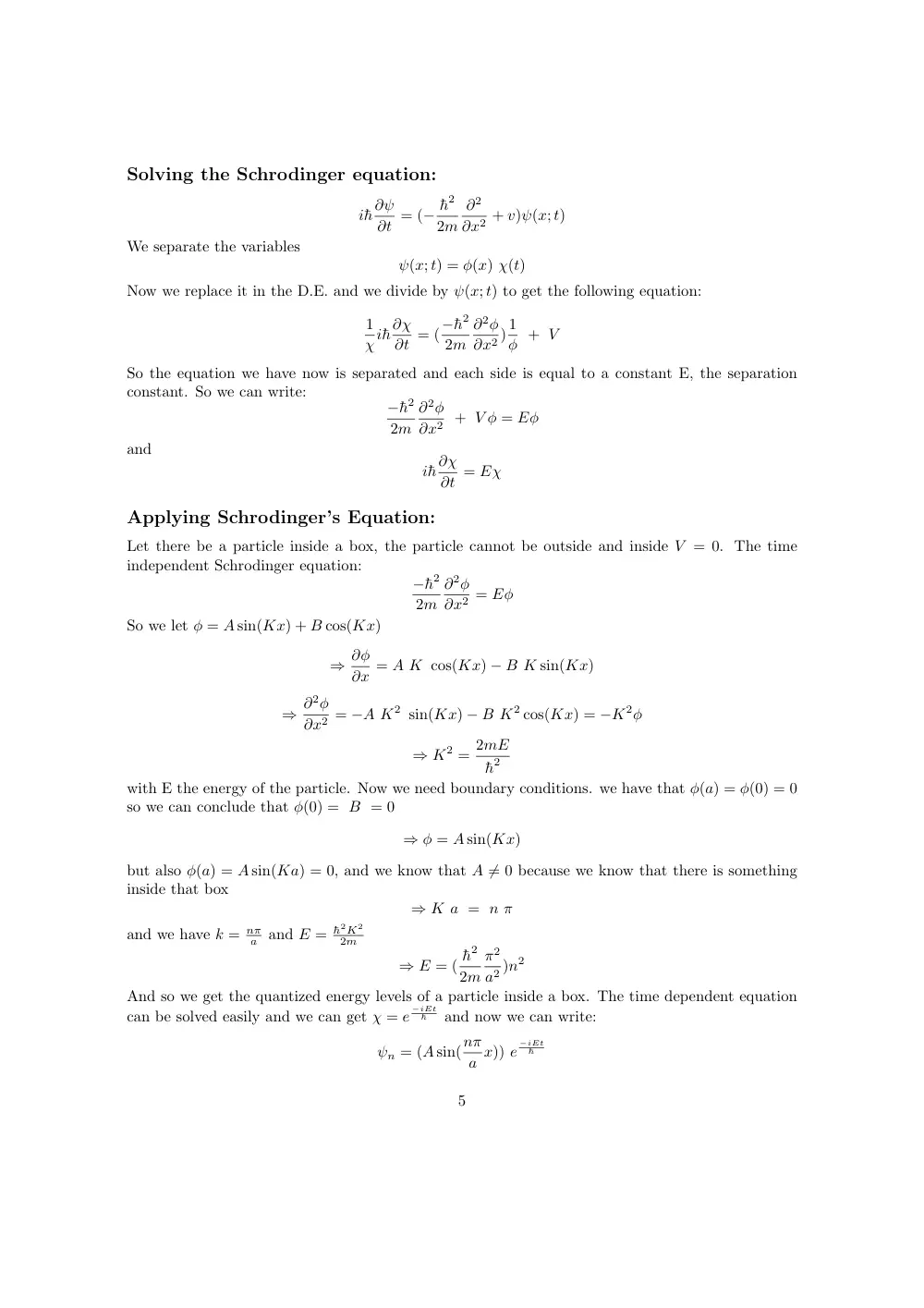Solving the Schrodinger equation: i¯h∂ψ ∂t = (− ¯h2 2m ∂2 ∂x2 + v)ψ(x; t) We separate the variables ψ(x; t) = φ(x) χ(t) Now we replace it in the D.E. and we divide by ψ(x; t) to get the following equation: 1 χi¯h∂χ ∂t = (−¯h2 2m ∂2φ ∂x2 ) 1 φ + V So the equation we have now is separated and each side is equal to a constant E, the separation constant. So we can write: −¯h2 2m ∂2φ ∂x2 + V φ = Eφ and i¯h∂χ ∂t = Eχ Applying Schrodinger’s Equation: Let there be a particle inside a box, the particle cannot be outside and inside V = 0. The time independent Schrodinger equation: −¯h2 2m ∂2φ ∂x2 = Eφ So we let φ = A sin(Kx) + B cos(Kx) ⇒ ∂φ ∂x = A K cos(Kx) − B K sin(Kx) ⇒ ∂2φ ∂x2 = −A K2 sin(Kx) − B K2 cos(Kx) = −K2φ ⇒ K2 = 2mE ¯h2 with E the energy of the particle. Now we need boundary conditions. we have that φ(a) = φ(0) = 0 so we can conclude that φ(0) = B = 0 ⇒ φ = A sin(Kx) but also φ(a) = A sin(Ka) = 0, and we know that A ̸= 0 because we know that there is something inside that box ⇒ K a = n π and we have k = nπ a and E = ¯h2K2 2m ⇒ E = ( ¯h2 2m π2 a2 )n2 And so we get the quantized energy levels of a particle inside a box. 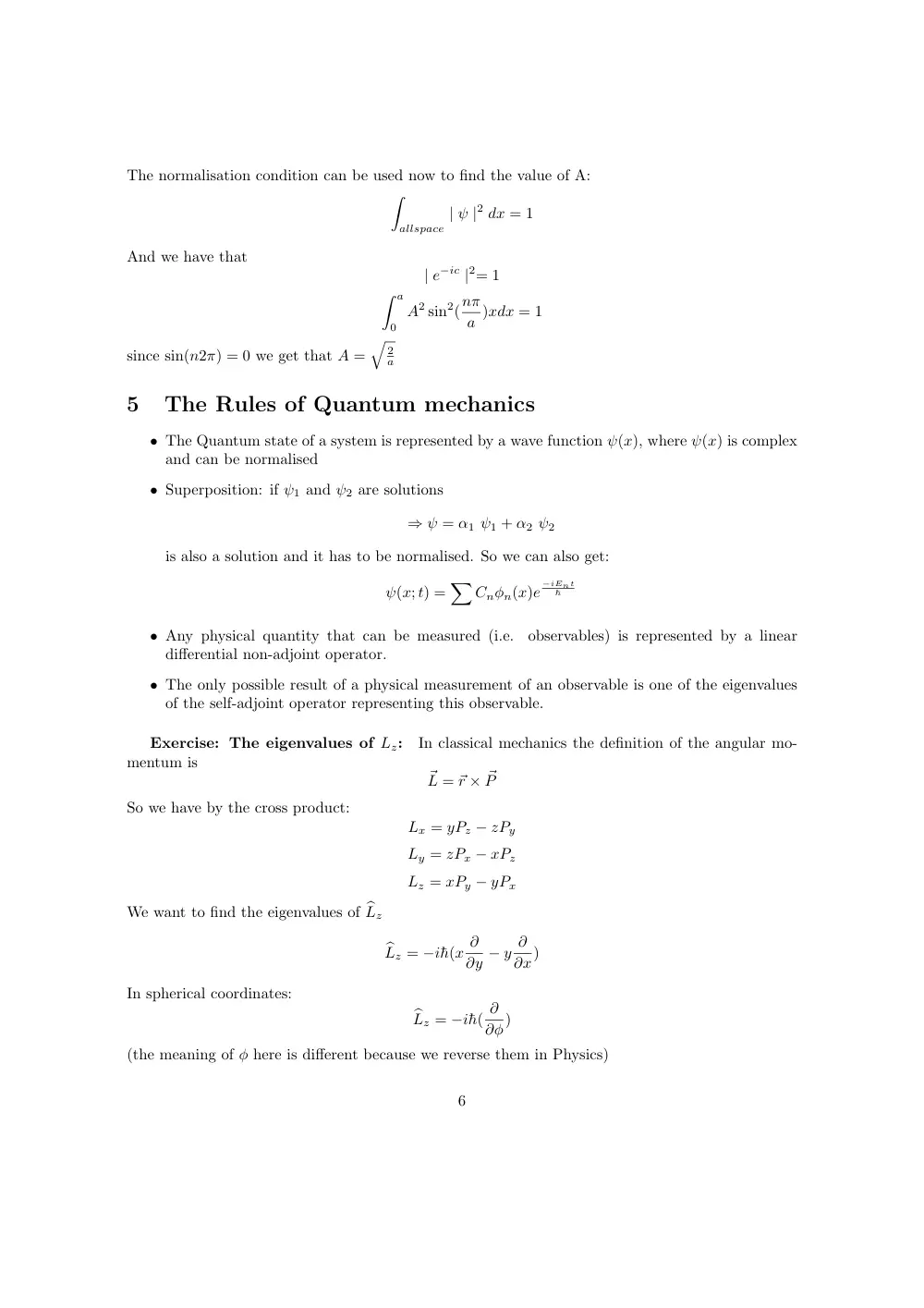The time dependent equation can be solved easily and we can get χ = e −iEt ¯h and now we can write: ψn = (A sin(nπ a x)) e −iEt ¯h 5 The normalisation condition can be used now to find the value of A: � allspace | ψ |2 dx = 1 And we have that | e−ic |2= 1 � a 0 A2 sin2(nπ a )xdx = 1 since sin(n2π) = 0 we get that A = � 2 a 5 The Rules of Quantum mechanics • The Quantum state of a system is represented by a wave function ψ(x), where ψ(x) is complex and can be normalised • Superposition: if ψ1 and ψ2 are solutions ⇒ ψ = α1 ψ1 + α2 ψ2 is also a solution and it has to be normalised. So we can also get: ψ(x; t) = � Cnφn(x)e −iEnt ¯h • Any physical quantity that can be measured (i.e. observables) is represented by a linear differential non-adjoint operator. • The only possible result of a physical measurement of an observable is one of the eigenvalues of the self-adjoint operator representing this observable. 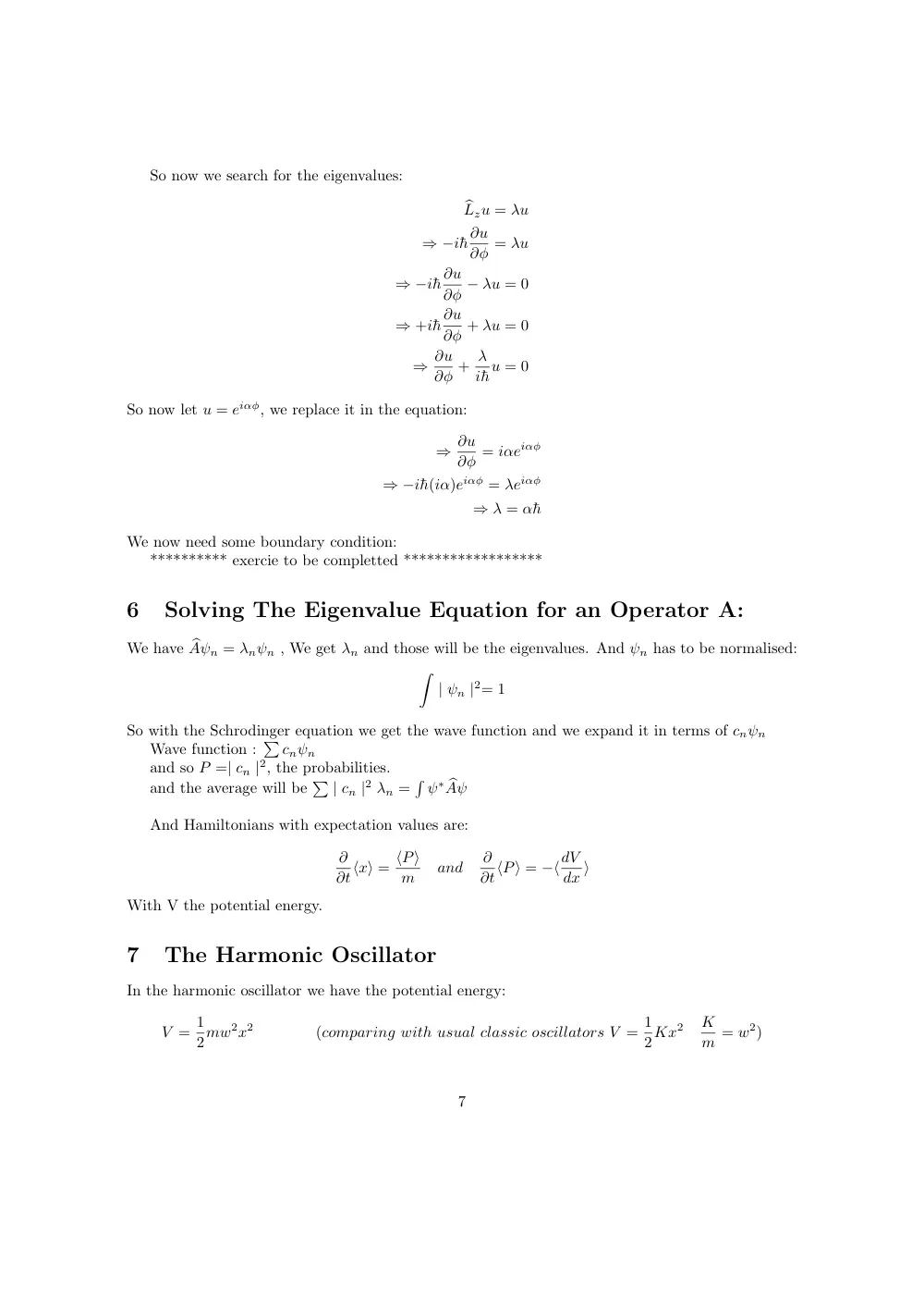Exercise: The eigenvalues of Lz: In classical mechanics the definition of the angular mo- mentum is ⃗L = ⃗r × ⃗P So we have by the cross product: Lx = yPz − zPy Ly = zPx − xPz Lz = xPy − yPx We want to find the eigenvalues of �Lz �Lz = −i¯h(x ∂ ∂y − y ∂ ∂x) In spherical coordinates: �Lz = −i¯h( ∂ ∂φ) (the meaning of φ here is different because we reverse them in Physics) 6 So now we search for the eigenvalues: �Lzu = λu ⇒ −i¯h∂u ∂φ = λu ⇒ −i¯h∂u ∂φ − λu = 0 ⇒ +i¯h∂u ∂φ + λu = 0 ⇒ ∂u ∂φ + λ i¯hu = 0 So now let u = eiαφ, we replace it in the equation: ⇒ ∂u ∂φ = iαeiαφ ⇒ −i¯h(iα)eiαφ = λeiαφ ⇒ λ = α¯h We now need some boundary condition: ********** exercie to be completted ****************** 6 Solving The Eigenvalue Equation for an Operator A: We have �Aψn = λnψn , We get λn and those will be the eigenvalues. And ψn has to be normalised: � | ψn |2= 1 So with the Schrodinger equation we get the wave function and we expand it in terms of cnψn Wave function : � cnψn and so P =| cn |2, the probabilities. and the average will be � | cn |2 λn = � ψ∗ �Aψ And Hamiltonians with expectation values are: ∂ ∂t⟨x⟩ = ⟨P⟩ m and ∂ ∂t⟨P⟩ = −⟨dV dx ⟩ With V the potential energy. 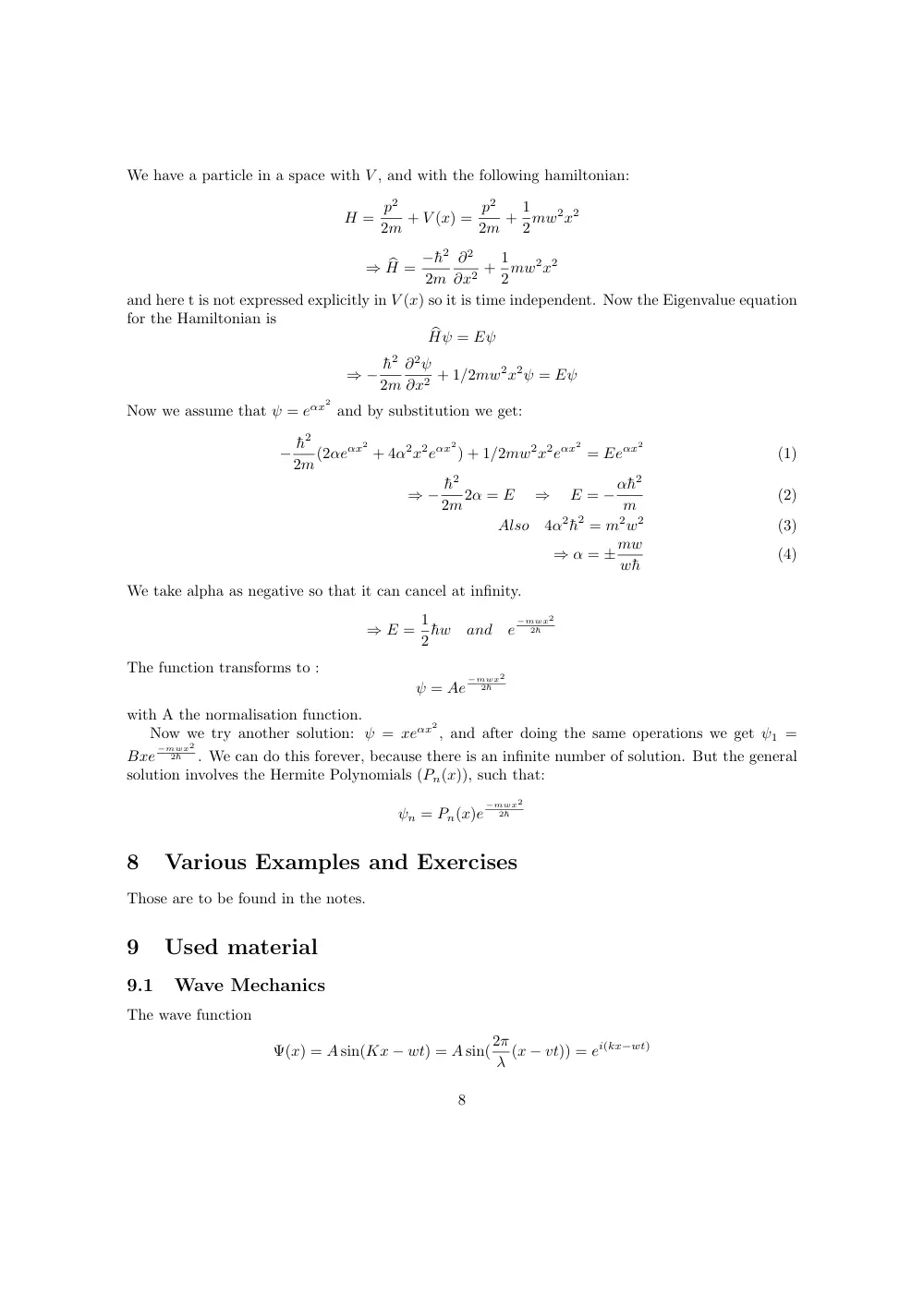7 The Harmonic Oscillator In the harmonic oscillator we have the potential energy: V = 1 2mw2x2 (comparing with usual classic oscillators V = 1 2Kx2 K m = w2) 7 We have a particle in a space with V , and with the following hamiltonian: H = p2 2m + V (x) = p2 2m + 1 2mw2x2 ⇒ �H = −¯h2 2m ∂2 ∂x2 + 1 2mw2x2 and here t is not expressed explicitly in V (x) so it is time independent. Now the Eigenvalue equation for the Hamiltonian is �Hψ = Eψ ⇒ − ¯h2 2m ∂2ψ ∂x2 + 1/2mw2x2ψ = Eψ Now we assume that ψ = eαx2 and by substitution we get: − ¯h2 2m(2αeαx2 + 4α2x2eαx2) + 1/2mw2x2eαx2 = Eeαx2 (1) ⇒ − ¯h2 2m2α = E ⇒ E = −α¯h2 m (2) Also 4α2¯h2 = m2w2 (3) ⇒ α = ±mw w¯h (4) We take alpha as negative so that it can cancel at infinity. ⇒ E = 1 2¯hw and e −mwx2 2¯h The function transforms to : ψ = Ae −mwx2 2¯h with A the normalisation function. Now we try another solution: ψ = xeαx2, and after doing the same operations we get ψ1 = Bxe −mwx2 2¯h . We can do this forever, because there is an infinite number of solution. But the general solution involves the Hermite Polynomials (Pn(x)), such that: ψn = Pn(x)e −mwx2 2¯h 8 Various Examples and Exercises Those are to be found in the notes. 9 Used material 9.1 Wave Mechanics The wave function Ψ(x) = A sin(Kx − wt) = A sin(2π λ (x − vt)) = ei(kx−wt) 8 Where v is the propagation velocity, w is the angular frequency w = v2π λ = 2πν , and A is the amplitude. And we also have ∂2ψ ∂x2 − 1 v2 ∂2ψ ∂t2 (5) Also we can describe the movement of the whole phase or group of waves ( or wave packets ) by the group velocity vg = dw dk 9.2 Eigenvalues A number ”a” is an eigenvalue of a differential operator �A if it satisfies the differential equation: �Au(x) = au(x) If A has un(x) as eigenfunctions with eigenvalues λn and suppose the wave function of the system is given by ψ(x) then ψ(x) = � n cnun(x) with Prob(λn) =| cn |2 9.3 Hermitian operators A self-adjoint (Hermitian) operator is an operator, such that: � −∞ ∞ [ �Aψ(x)]∗ φ(x)dx = � −∞ ∞ ψ∗(x) [ �Aφ(x)]dx 9.4 Average of an observable To find the average value of an observable after multiple observations, we do this calculation: ⟨A⟩ = � allspace ψ∗ �Aψ = � i λi | ci |2 9.5 Hermite Polynomials A hermite polynomial is the one that is the sum of a certain order of x multiplied by coefficients, but if the order is odd the only possible orders are odd, and if it even, the same is applied. 9