STAT 210 Lecture Chapter 2, Fall 2015

CHAPTER 2 ORGANIZING AND GRAPHING DATA Prem Mann, Introductory Statistics, 8/E Copyright © 2013 John Wiley & Sons. All rights reserved. RAW DATA  Definition  Data recorded in the sequence in which they are collected and before they are processed or ranked are called raw data.  ORGANIZING AND GRAPHING DATA: • Frequency Distributions • Relative Frequency and Percentage Distributions • Graphical Presentation of Qualitative Data Prem Mann, Introductory Statistics, 8/E Copyright © 2013 John Wiley & Sons. All rights reserved. Table 2.3 Types of Employment Students Intend to Engage In Prem Mann, Introductory Statistics, 8/E Copyright © 2013 John Wiley & Sons. All rights reserved. Frequency Distributions  Definition  A frequency distribution of a qualitative variable lists all categories and the number of elements that belong to each of the categories. Prem Mann, Introductory Statistics, 8/E Copyright © 2013 John Wiley & Sons. All rights reserved. Relative Frequency and Percentage Distributions  Calculating Relative Frequency of a Category of all frequencies Sum Frequency of that category Re lative frequency of a category  Prem Mann, Introductory Statistics, 8/E Copyright © 2013 John Wiley & Sons. All rights reserved. Calculating Percentage Percentage = (Relative frequency) · 100% Graphical Presentation of Qualitative Data  Definition  A graph made of bars whose heights represent the frequencies of respective categories is called a bar graph. Prem Mann, Introductory Statistics, 8/E Copyright © 2013 John Wiley & Sons. All rights reserved. ORGANIZING AND GRAPHING QUANTITATIVE • Frequency Distributions • Constructing Frequency Distribution Tables • Relative and Percentage Distributions • Graphing Grouped Data Prem Mann, Introductory Statistics, 8/E Copyright © 2013 John Wiley & Sons. All rights reserved. 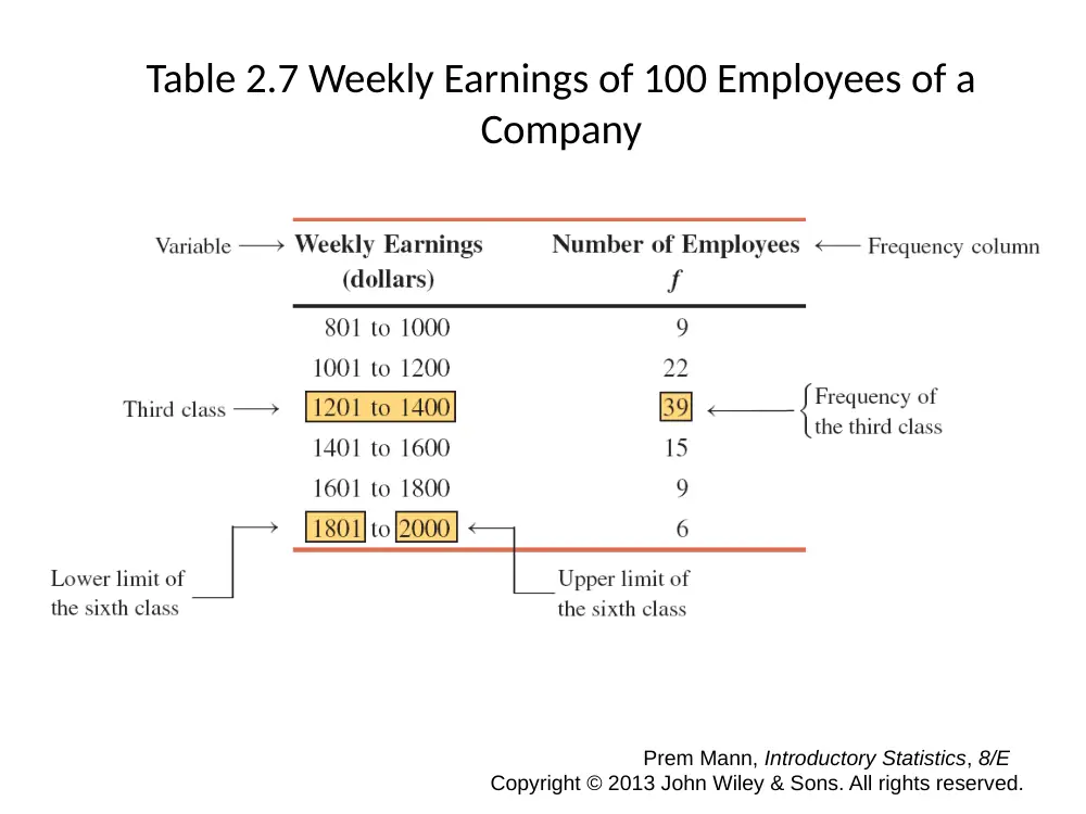Table 2.7 Weekly Earnings of 100 Employees of a Company Prem Mann, Introductory Statistics, 8/E Copyright © 2013 John Wiley & Sons. All rights reserved. Frequency Distributions  Definition  A frequency distribution for quantitative data lists all the classes and the number of values that belong to each class. Data presented in the form of a frequency distribution are called grouped data. Prem Mann, Introductory Statistics, 8/E Copyright © 2013 John Wiley & Sons. All rights reserved. Frequency Distributions  Definition  The class boundary is given by the midpoint of the upper limit of one class and the lower limit of the next class. Finding Class Width Class width = Upper boundary – Lower boundary Prem Mann, Introductory Statistics, 8/E Copyright © 2013 John Wiley & Sons. All rights reserved. Frequency Distributions Calculating Class Midpoint or Mark 2 Lower limit Upper limit Class midpoint or mark   Prem Mann, Introductory Statistics, 8/E Copyright © 2013 John Wiley & Sons. All rights reserved. Table 2.8 Class Boundaries, Class Widths, and Class Midpoints for Table 2.7 Prem Mann, Introductory Statistics, 8/E Copyright © 2013 John Wiley & Sons. All rights reserved. Graphing Grouped Data  Definition  A histogram is a graph in which classes are marked on the horizontal axis and the frequencies, relative frequencies, or percentages are marked on the vertical axis. The frequencies, relative frequencies, or percentages are represented by the heights of the bars. In a histogram, the bars are drawn adjacent to each other. Prem Mann, Introductory Statistics, 8/E Copyright © 2013 John Wiley & Sons. All rights reserved. Table 2.9 Frequency Distribution for the Data on iPods Sold Prem Mann, Introductory Statistics, 8/E Copyright © 2013 John Wiley & Sons. All rights reserved. Figure 2.3 Frequency histogram for Table 2.9. Prem Mann, Introductory Statistics, 8/E Copyright © 2013 John Wiley & Sons. All rights reserved. Graphing Grouped Data  Definition  A graph formed by joining the midpoints of the tops of successive bars in a histogram with straight lines is called a polygon. Prem Mann, Introductory Statistics, 8/E Copyright © 2013 John Wiley & Sons. All rights reserved. Figure 2.5 Frequency polygon for Table 2.9. Prem Mann, Introductory Statistics, 8/E Copyright © 2013 John Wiley & Sons. All rights reserved. Example 2-6 The administration in a large city wanted to know the distribution of vehicles owned by households in that city. A sample of 40 randomly selected households from this city produced the following data on the number of vehicles owned: 5 1 1 2 0 1 1 2 1 1 1 3 3 0 2 5 1 2 3 4 2 1 2 2 1 2 2 1 1 1 4 2 1 1 2 1 1 4 1 3 Construct a frequency distribution table for these data using single-valued classes. Prem Mann, Introductory Statistics, 8/E Copyright © 2013 John Wiley & Sons. All rights reserved. Example 2-6: Solution Table 2.13 Frequency Distribution of Vehicles Owned The observations assume only six distinct values: 0, 1, 2, 3, 4, and 5. Each of these six values is used as a class in the frequency distribution in Table 2.13. Prem Mann, Introductory Statistics, 8/E Copyright © 2013 John Wiley & Sons. All rights reserved. Figure 2.7 Bar graph for Table 2.13. Prem Mann, Introductory Statistics, 8/E Copyright © 2013 John Wiley & Sons. All rights reserved. SHAPES OF HISTOGRAMS 1. Symmetric 2. Skewed 3. Uniform or Rectangular Prem Mann, Introductory Statistics, 8/E Copyright © 2013 John Wiley & Sons. All rights reserved. Figure 2.8 Symmetric histograms. Prem Mann, Introductory Statistics, 8/E Copyright © 2013 John Wiley & Sons. All rights reserved. Figure 2.9 (a) A histogram skewed to the right. (b) A histogram skewed to the left. Prem Mann, Introductory Statistics, 8/E Copyright © 2013 John Wiley & Sons. All rights reserved. Figure 2.10 A histogram with uniform distribution. Prem Mann, Introductory Statistics, 8/E Copyright © 2013 John Wiley & Sons. All rights reserved. CUMULATIVE FREQUENCY DISTRIBUTIONS  Definition  A cumulative frequency distribution gives the total number of values that fall below the upper boundary of each class. Prem Mann, Introductory Statistics, 8/E Copyright © 2013 John Wiley & Sons. All rights reserved. Example 2-7: Solution Table 2.14 Cumulative Frequency Distribution of iPods Sold Prem Mann, Introductory Statistics, 8/E Copyright © 2013 John Wiley & Sons. All rights reserved. CUMULATIVE FREQUENCY DISTRIBUTIONS  Calculating Cumulative Relative Frequency and Cumulative Percentage percentage (Cumulativ e relative frequency) 100 Cumulative observations in the data set Total Cumulative frequency of a class relative frequency Cumulative    Prem Mann, Introductory Statistics, 8/E Copyright © 2013 John Wiley & Sons. All rights reserved. Figure 2.12 Ogive for the cumulative frequency distribution of Table 2.14. Prem Mann, Introductory Statistics, 8/E Copyright © 2013 John Wiley & Sons. All rights reserved. STEM-AND-LEAF DISPLAYS  Definition  In a stem-and-leaf display of quantitative data, each value is divided into two portions – a stem and a leaf. The leaves for each stem are shown separately in a display. Prem Mann, Introductory Statistics, 8/E Copyright © 2013 John Wiley & Sons. All rights reserved. Example 2-8  The following are the scores of 30 college students on a statistics test:  Construct a stem-and-leaf display. 75 69 83 52 72 84 80 81 77 96 61 64 65 76 71 79 86 87 71 79 72 87 68 92 93 50 57 95 92 98 Prem Mann, Introductory Statistics, 8/E Copyright © 2013 John Wiley & Sons. All rights reserved. Figure 2.13 Stem-and-leaf display. Prem Mann, Introductory Statistics, 8/E Copyright © 2013 John Wiley & Sons. All rights reserved. Figure 2.14 Stem-and-leaf display of test scores. Prem Mann, Introductory Statistics, 8/E Copyright © 2013 John Wiley & Sons. All rights reserved.