ECO 226 Problems Chapter 3 Solution, Spring 2017

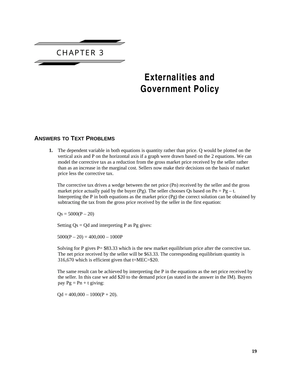
CHAPTER 3 Externalities and Government Policy ANSWERS TO TEXT PROBLEMS 1. The dependent variable in both equations is quantity rather than price. Q would be plotted on the vertical axis and P on the horizontal axis if a graph were drawn based on the 2 equations. We can model the corrective tax as a reduction from the gross market price received by the seller rather than as an increase in the marginal cost. Sellers now make their decisions on the basis of market price less the corrective tax. The corrective tax drives a wedge between the net price (Pn) received by the seller and the gross market price actually paid by the buyer (Pg). The seller chooses Qs based on Pn = Pg – t. Interpreting the P in both equations as the market price (Pg) the correct solution can be obtained by subtracting the tax from the gross price received by the seller in the first equation: Qs = 5000(P – 20) Setting Qs = Qd and interpreting P as Pg gives: 5000(P – 20) = 400,000 – 1000P Solving for P gives P= $83.33 which is the new market equilibrium price after the corrective tax. The net price received by the seller will be $63.33. The corresponding equilibrium quantity is 316,670 which is efficient given that t=MEC=$20. The same result can be achieved by interpreting the P in the equations as the net price received by the seller. In this case we add $20 to the demand price (as stated in the answer in the IM). Buyers pay Pg = Pn + t giving: Qd = 400,000 – 1000(P + 20). 19 20 | Part One | The Economic Basis of Government Activity Setting Qs = Qd and interpreting P and Pn gives: 400,000 – 1000(P + 20) = 5000P Solving this gives a net price of $63.33, which implies a market equilibrium price after the tax is added of $83.33—the same as above. 2. The demand curve is obtained by plotting the data for MPB on the vertical axis and plotting the quantity on the horizontal axis. The difference between the marginal social benefit and the margi- nal private benefit is the MEB. At a price of $25 per gallon, the market equilibrium is not efficient because there is a marginal external benefit of $6 when 30 million gallons are sold per year. At a $15 price, the marginal external benefit is zero, and the market equilibrium is therefore efficient. 3. a. The cost of meeting the standards is obtained by multiplying cost per ton for each plant and summing the results, which gives $220,000 per year. b. The least cost method would be to have Plant 5 reduce its emissions by 500 tons per year, which would cost only $100,000 per year. 4. At a $450 per ton charge, Plants 4 and 5 would cut back emissions at a total cost of $60,000. Plants 1, 2, and 3 would find it cheaper to pay the $450 fee, rather than cut back emissions. The total reve- nue generated by the purchase of the pollution rights by these firms for the 300-ton reduction in annual emissions would therefore be $135,000. 5. The efficient amount of pollution abatement occurs at the point at which the marginal social cost of abatement is equal to its marginal social benefit. Because the marginal social cost rises while the marginal social benefit declines, the efficient amount of abatement is likely to be greater than zero but less than 100 percent. In practice it is difficult to determine the efficient level of pollution abate- ment because of difficulty in assessing the costs and benefits of abating pollution and the way they vary at the margin as more abatement is achieved. © 2011 Cengage Learning. All Rights Reserved. May not be scanned, copied or duplicated, or posted to a publicly accessible website, in whole or in part.