INDE 301 Lecture All Notes, Spring 2016

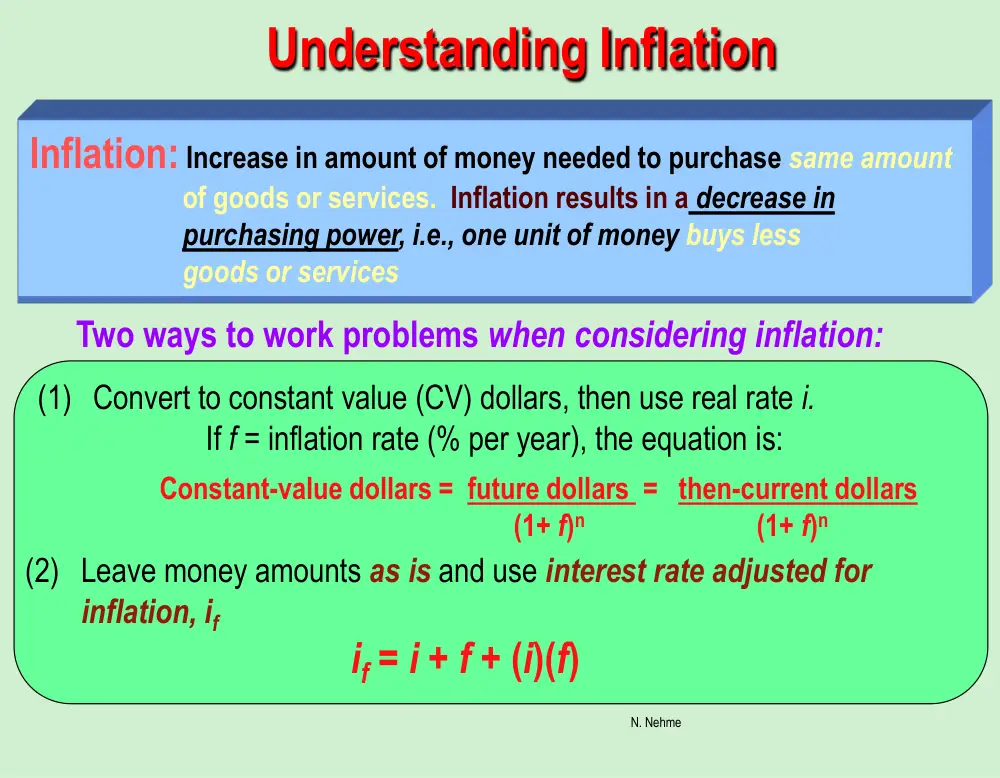
INDE 301 Engineering Economy Effects of Inflation Review and Examples © 2012 by McGraw-Hill, New York, N.Y Dr. N. Nehme Understanding Inflation Inflation: Increase in amount of money needed to purchase same amount of goods or services. Inflation results in a decrease in purchasing power, i.e., one unit of money buys less goods or services Constant-value dollars = future dollars = then-current dollars (1+ f)n (1+ f)n (1) Convert to constant value (CV) dollars, then use real rate i. If f = inflation rate (% per year), the equation is: (2) Leave money amounts as is and use interest rate adjusted for inflation, if if = i + f + (i)(f) Two ways to work problems when considering inflation: N. 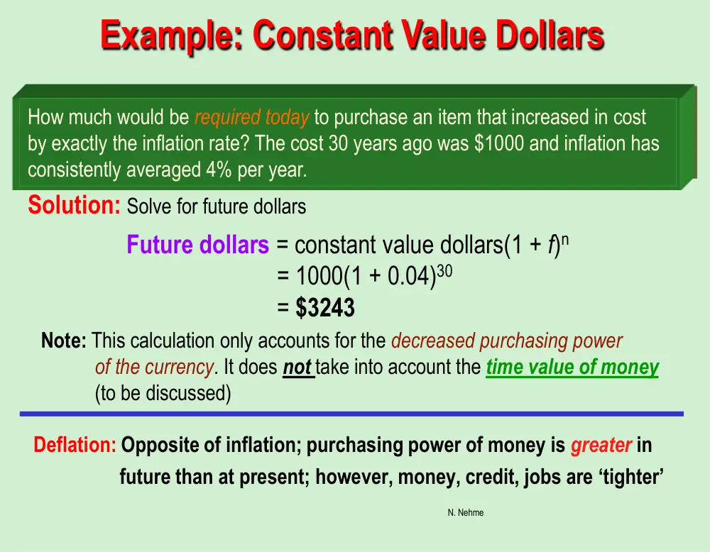Nehme Example: Constant Value Dollars Solution: Solve for future dollars How much would be required today to purchase an item that increased in cost by exactly the inflation rate? The cost 30 years ago was $1000 and inflation has consistently averaged 4% per year. Future dollars = constant value dollars(1 + f)n = 1000(1 + 0.04)30 = $3243 Note: This calculation only accounts for the decreased purchasing power of the currency. It does not take into account the time value of money (to be discussed) Deflation: Opposite of inflation; purchasing power of money is greater in future than at present; however, money, credit, jobs are ‘tighter’ N. 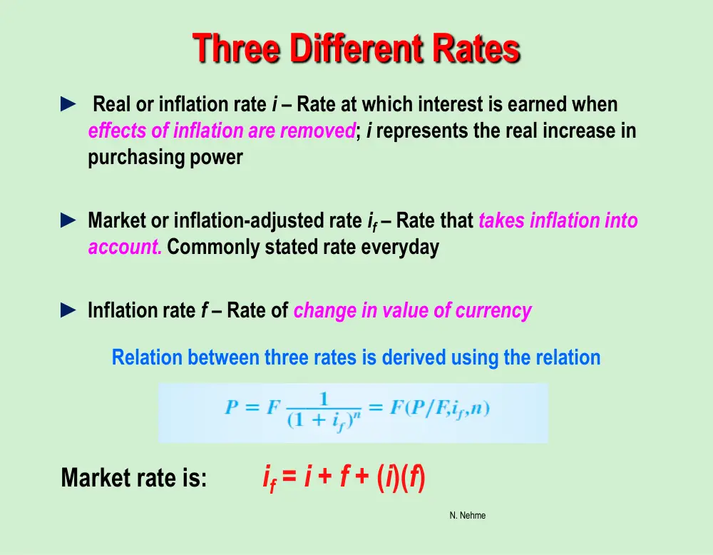Nehme Three Different Rates ► Real or inflation rate i – Rate at which interest is earned when effects of inflation are removed; i represents the real increase in purchasing power ► Market or inflation-adjusted rate if – Rate that takes inflation into account. Commonly stated rate everyday ► Inflation rate f – Rate of change in value of currency Relation between three rates is derived using the relation Market rate is: if = i + f + (i)(f) N. 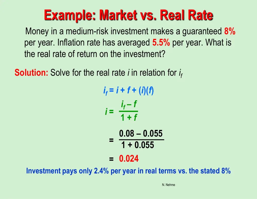Nehme Example: Market vs. Real Rate Money in a medium-risk investment makes a guaranteed 8% per year. Inflation rate has averaged 5.5% per year. What is the real rate of return on the investment? Solution: Solve for the real rate i in relation for if if = i + f + (i)(f) if – f 1 + f 0.08 – 0.055 1 + 0.055 0.024 Investment pays only 2.4% per year in real terms vs. the stated 8% i = = = N. 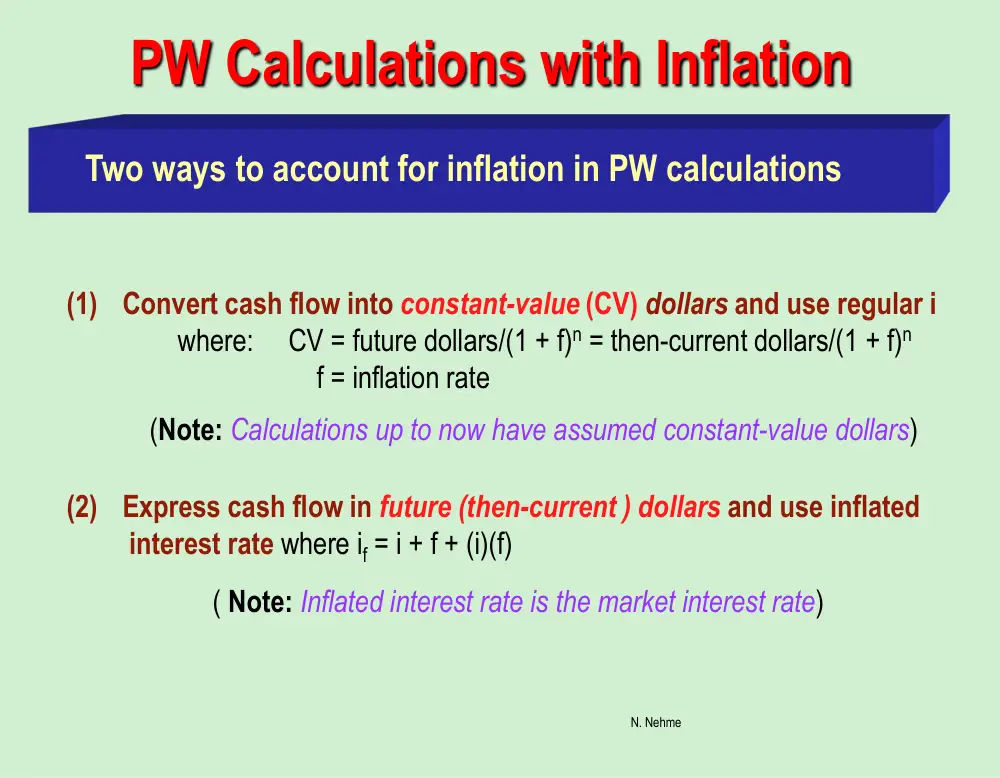Nehme PW Calculations with Inflation Two ways to account for inflation in PW calculations (2) Express cash flow in future (then-current ) dollars and use inflated interest rate where if = i + f + (i)(f) ( Note: Inflated interest rate is the market interest rate) (1) Convert cash flow into constant-value (CV) dollars and use regular i where: CV = future dollars/(1 + f)n = then-current dollars/(1 + f)n f = inflation rate (Note: Calculations up to now have assumed constant-value dollars) N. 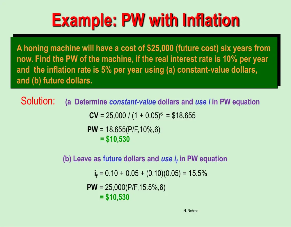Nehme Example: PW with Inflation A honing machine will have a cost of $25,000 (future cost) six years from now. Find the PW of the machine, if the real interest rate is 10% per year and the inflation rate is 5% per year using (a) constant-value dollars, and (b) future dollars. CV = 25,000 / (1 + 0.05)6 = $18,655 PW = 18,655(P/F,10%,6) = $10,530 Solution: (a Determine constant-value dollars and use i in PW equation (b) Leave as future dollars and use if in PW equation if = 0.10 + 0.05 + (0.10)(0.05) = 15.5% PW = 25,000(P/F,15.5%,6) = $10,530 N. Nehme FW Calculations with Inflation FW values can have four different interpretations (2) The purchasing power in terms of CV dollars of the future amount  Use if in FW equation and divide by (1+f)n or use real i where real i = (if – f)/(1 + f) FW = PW(F/P,i,n) (3) The number of future dollars required to have the same purchasing power as a dollar today with no time value of money considered  Use f instead of i in F/P factor FW = PW(F/P,f,n) (1) The actual amount accumulated  Use if in FW equation FW = PW(F/P, if, n) (4) The amount required to maintain the purchasing power of the present sum and earn a stated real rate of return  Use if in FW equation FW = PW(F/P, if, n) N. 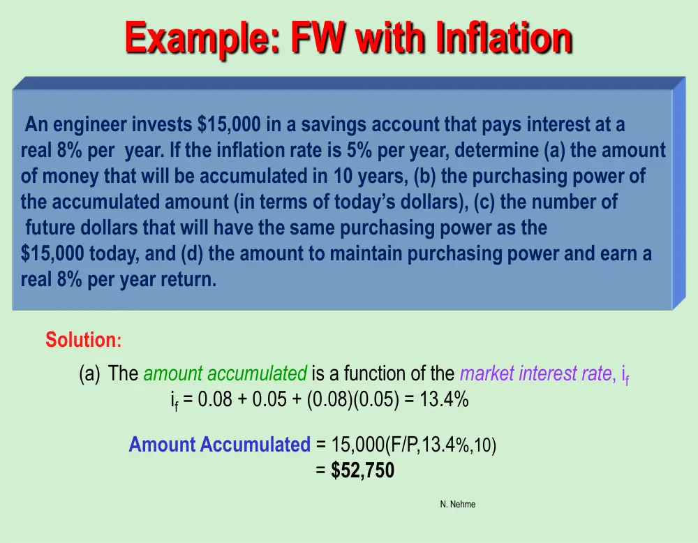Nehme Example: FW with Inflation An engineer invests $15,000 in a savings account that pays interest at a real 8% per year. If the inflation rate is 5% per year, determine (a) the amount of money that will be accumulated in 10 years, (b) the purchasing power of the accumulated amount (in terms of today’s dollars), (c) the number of future dollars that will have the same purchasing power as the $15,000 today, and (d) the amount to maintain purchasing power and earn a real 8% per year return. (a) The amount accumulated is a function of the market interest rate, if if = 0.08 + 0.05 + (0.08)(0.05) = 13.4% Amount Accumulated = 15,000(F/P,13.4%,10) = $52,750 Solution: N. Nehme Example: FW with Inflation (cont’d) (c) The number of future dollars required to purchase goods that cost $15,000 now is the inflated cost of the goods Number of future dollars = 15,000(F/P,5%,10) = $24,434 (b) To find the purchasing power of the accumulated amount deflate the inflated dollars Purchasing power = 15,000(F/P,13.4%,10) / (1 + 0.05)10 = $32,384 (d) In order to maintain purchasing power and earn a real return, money must grow by the inflation rate and the interest rate, or if = 13.4%, as in part (a) FW = 15,000(F/P,13.4%,10) = $52,750 N. Nehme Capital Recovery with Inflation The A/P and A/F factors require the use of if when inflation is considered If a small company invests $150,000 in a new production line machine, how much must it receive each year to recover the investment in 5 years? The real interest rate is 10% and the inflation rate is 4% per year. Solution: Capital recovery (CR) is the AW value if = 0.10 + 0.04 + (0.10)(0.04) = 14.4% CR = AW = 150,000(A/P,14.4%,5) = $44,115 per year N. Nehme INDE 301 Engineering Economy Depreciation Methods © 2012 by McGraw-Hill, New York, N.Y Dr. N. Nehme 1. Understand basic terms of asset depreciation 2. Apply straight line method of depreciation 3. Apply DB and DDB methods of depreciation; switch between DDB and SL methods 4. Explain depletion and apply cost depletion & percentage depletion methods © 2012 by McGraw-Hill All Rights Reserved Dr. N. Nehme © 2012 by McGraw-Hill All Rights Reserved Dr. N. Nehme Depreciation Terminology Definition: Book (noncash) method to represent decrease in value of a tangible asset over time Two types: book depreciation and tax depreciation Book depreciation: used for internal accounting to track value of assets Tax depreciation: used to determine taxes due based on tax laws 4 Common Depreciation Terms © 2012 by McGraw-Hill All Rights Reserved Dr. N. Nehme First cost P or unadjusted basis B: Total installed cost of asset Book value BVt: Remaining undepreciated capital investment in year t Recovery period n: Depreciable life of asset in years Market value MV: Amount realizable if asset were sold on open market Salvage value S: Estimated trade-in or MV at end of asset’s useful life Depreciation rate dt: Fraction of first cost or basis removed each year t Personal property: Possessions of company used to conduct business Real property: Real estate and all improvements (land is not depreciable) Half-year convention: Assumes assets are placed in service in midyear Straight Line Depreciation © 2012 by McGraw-Hill All Rights Reserved Dr. N. Nehme Book value decreases linearly with time Dt = B - S n Where: Dt = annual depreciation charge t = year B = first cost or unadjusted basis S = salvage value n = recovery period BVt = B - tDt Where: BVt = book value after t years SL depreciation rate is constant for each year: d = dt = 1/n 6 Example: SL Depreciation © 2012 by McGraw-Hill All Rights Reserved Dr. N. Nehme Solution: (a ) D3 = (B – S)/n = (20,000 – 5,000)/5 = $3,000 (b) BV3 = B – tDt = 20,000 – 3(3,000) = $11,000 An argon gas processor has a first cost of $20,000 with a $5,000 salvage value after 5 years. Find (a) D3 and (b) BV3 for year three. (c) Plot book value vs. time. (c) Plot BV vs. time 20,000 11,000 3 5 5,000 0 Year, t BVt 7 Declining Balance (DB) and Double Declining Balance (DDB) Depreciation © 2012 by McGraw-Hill All Rights Reserved Dr. N. Nehme Determined by multiplying BV at beginning of year by fixed percentage d Max rate for d is twice straight line rate, i.e., d ≤ 2/n Cannot depreciate below salvage value Depreciation for year t is obtained by either relation: Dt = dB(1 – d)t-1 = dBVt-1 Where: Dt = depreciation for year t d = uniform depreciation rate (2/n for DDB) B = first cost or unadjusted basis BVt -1 = book value at end of previous year Book value for year t is given by: BVt = B(1 – d)t 8 Example: Double Declining Balance © 2012 by McGraw-Hill All Rights Reserved Dr. N. Nehme (b) BV3 = B(1 – d)t = 20,000(1 – 0.4)3 = $4320 A depreciable construction truck has a first cost of $20,000 with a $4,000 salvage value after 5 years. Find the (a) depreciation, and (b) book value after 3 years using DDB depreciation. Solution: (a) d = 2/n = 2/5 = 0.4 D3 = dB(1 – d)t-1 = 0.4(20,000)(1 – 0.40)3-1 = $2880 9 Spreadsheet Functions for Depreciation © 2012 by McGraw-Hill All Rights Reserved Dr. N. Nehme Straight line function: SLN(B,S,n) Declining balance function: DB(B,S,n,t) Double declining balance function: DDB(B,S,n,t,d) Note: It is better to use the DDB function for DB and DDB depreciation. DDB function checks for BV < S and is more accurate than the DB function. 10 © 2012 by McGraw-Hill All Rights Reserved Dr. N. Nehme Depletion Methods Depletion: book (noncash) method to represent decreasing value of natural resources Two methods: cost depletion (CD) and percentage depletion (PD) Cost depletion: Based on level of activity to remove a natural resource  Calculation: Multiply factor CDt by amount of resource removed Where: CDt = first cost / resource capacity  Total depletion can not exceed first cost of the resource Percentage depletion: Based on gross income (GI) from resource  Calculation: Multiply GI by standardized rate (%) from table  Annual depletion can not exceed 50% of company’s taxable income (TI) © 2012 by McGraw-Hill All Rights Reserved Dr. N. Nehme 11 Example: Cost and Percentage Depletion A mine purchased for $3.5 million has a total expected yield of one million ounces of silver. Determine the depletion charge in year 4 when 300,000 ounces are mined and sold for $30 per ounce using (a) cost depletion, and (b) percentage depletion. (c) Which is larger for year 4? Solution: Let depletion amounts equal CDA4 and PDA4 (a) Factor, CD4 = 3,500,000/ 1,000,000 = $3.50 per ounce CDA4 = 3.50(300,000) = $1,050,000 (b) Percentage depletion rate for silver mines is 0.15 PDA4 = (0.15)(300,000)(30) = $1,350,000 (c) Claim percentage depletion amount, provided it is ≤ 50% of TI N. Nehme Engineering Economy Page 1 of 13 INDE 301 Engineering Economy Introduction to Accounting and Setting the MARR1  What is accounting?  Accounting is the act of gathering and reporting the financial history of an organization (company).  This requires a continuous process of o Capturing financial data, o Organizing it, o Producing financial reports.  Framework for understanding accounting information  Information in accounting reports are determined by o Economic concepts. Determine what is being actually reported? E.g., financial value, wealth, income. o Accounting conventions. Dictate how to report financial transactions to measure the desired economic criteria. o Institutional context. This reflects the effect of human judgment in adopting accounting conventions. 1 Compiled mostly from Antle and Gartska (2004), Financial Accounting, and Chapter 10, text. N. Nehme Engineering Economy Page 2 of 13  Financial Statements: Balance Sheet  An organization’s balance sheet is a list of resources available (assets), resources committed (liabilities), and their difference (equity) at a point in time.  The numbers on the balance sheet add up. Assets and liabilities and stockholders' equity must balance.  This is the fundamental accounting identity, ASSETS = LIABILITIES + EQUITY .  Equivalently, ASSETS – LIABILITIES = EQUITY . N. Nehme Engineering Economy Page 3 of 13  Financial Statements: Income Statement  An organization’s income statement lists the economic resources acquired (revenues) and consumed (expenses) through operations over a period of time.  The income statement reports success or failure of company's operations during the period.  Relative to the balance sheet, the income statement explains the change in retained earnings between the beginning and end of the period. N. Nehme Engineering Economy Page 4 of 13  Financial Statements: Cash Flow Statement  An organization’s cash flow statement describes flow of cash into and out of organization during a period.  The cash flows are classified as one of three types o Operating activities. Intended to generate net income. o Investing activities. Resulting from acquiring or disposing of productive company assets. o Financing activities. Payments to or receipts from suppliers of money (e.g., shareholders or debt holders).  Relative to the balance sheet, the income statement explains the change in cash between the beginning and end of period. N. Nehme Engineering Economy Page 5 of 13  Annual Report  The balance sheet, the income statement and the cash flow statement are part of a comprehensive financial report called annual report.  The annual report contains other elements such as the retained earnings statement, management discussion and analysis, notes to financial statements and auditor’s report.  Balance Sheet Contents  A balance sheet generally contains the following: o Current assets o Noncurrent assets o Current Liabilities o Noncurrent (long-term) liabilities o Stockholders' equity  Assets  An asset (i) generates economic benefit, (ii) is owned or controlled, (iii) is the result of a past transaction.  Current assets are converted to cash or used in business within one year. E.g., cash, short-term investments, accounts receivable, and inventories. N. Nehme Engineering Economy Page 6 of 13  Noncurrent assets are converted to cash or used in business after more than one year. E.g., property, plant and equipment, long-term investments, and rights.  An asset market value is the value the market assigns to an asset.  Book value is the value accounting assigns to an asset.  Market value and book value are often different.  Depreciation is the deduction of the book value over time.  Liabilities  A liability (i) requires a future sacrifice, (ii) is an obligation, and (iii) is the result of a past transaction.  Current liabilities are expected to be paid within one year. E.g., accounts payable, accrued liabilities, short-term borrowings, dividends payable, unearned revenues.  Dividends are the part of earnings that a company shares with its shareholders (owners).  Noncurrent liabilities are debts expected to be paid after more than one year. E.g., warranties, employee benefits, lease, bonds payable, long-term borrowings. N. Nehme Engineering Economy Page 7 of 13  Stockholders' Equity  This is the difference between total assets and total liabilities, which arises from the contributions of owners and economic income.  Examples include o Common Stock. Shareholders’ investment in entity through acquisition of stock. Entitles holder to vote on major decisions and claim assets in case of liquidation. o Preferred stock. Similar to common stock. Owners are typically not allowed to vote on major decisions. They however have priority in dividend and claim on assets in case of liquidation. o Retained Earnings. Net income generated from operations less what has been returned to shareholders in dividends. N. Nehme Engineering Economy Page 8 of 13  Setting the MARR  As you have seen, the minimum attractive rate of return (MARR) is essential in engineering economic analysis.  As mentioned previously, the MARR is set above the company’s cost of capital.  The cost of capital is a weighted average of the cost of debt and equity financing.  In establishing the MARR, the company’s management adds increments for (i) additional return and (ii) risk factor.  The MARR may vary from one project to another and over time because of factors such as risk, investment opportunity, tax, capital limitation, competition. N. Nehme Engineering Economy Page 9 of 13  Weighted Average Cost of Capital (WACC)  Financing of a project comes from equity and debt sources.  WACC is estimated as follows WACC = (equity fraction)(cost of equity capital) + (debt fraction) (cost of debt capital)  Costs of equity and debt capitals are divided into several categories as reflected in the company’s balance sheet.  Debt financing is considered risky as it entails strict payment obligations to the company.  Debt-to-equity-ratio = liabilities/equities is used to assess the risk of debt financing. (Text refers to this ratio as D-E mix.)  Determining the Cost of Debt Capital  Debt financing is obtained mainly through loans and bonds.  Bond and loans interest payments are tax-deductible.  (For bonds, “interest” includes coupon payment and price discounts relative to the face value.) N. Nehme Engineering Economy Page 10 of 13  Tax deductible means that the interest payments will be considered “expenses” on the company’s income statement leading to a lower net income.  This leads to tax saving as taxes apply to net income.  This is an advantage of debt financing. (Do not forget that debt financing is risky though.)  The cost of debt capital is then found as the ROR (yield) of the bond or loan after adjusting down the interest expenses at the appropriate tax rate.  E.g., let Te be the tax rate, and suppose a company receives P now and pays Ct in interest in periods t =1, …, n and then pays P back at time n. (This is like a bond at par.)  Then, the cost of debt capital is id * that satisfies * * 1 (1 ) 0 (1 ) (1 ) n e t t n t d d T C P P i i         .  For bonds not at par, the analysis should include tax deduction from interest in terms of discount on face value, which is more involved.  Determining the Cost of Equity Capital  Equity financing comes from issuing preferred stock, and common stock, and from retained earnings.  Tax considerations do not affect equity cost of capital since stock dividends are not tax-deductible. N. Nehme Engineering Economy Page 11 of 13  Preferred stocks typically guarantee a stated dividend annually, quoted as a percentage of the par (issuance) value.2  This percentage can be used as the cost of capital for the preferred stock.  E.g. a 10% dividend preferred stock with a par value of $100, will pay an annual dividend of $10.  The cost of capital in this case is 10% .  For common stock, no stated rate of return is guaranteed.  One approach is to estimate the dividend growth rate, g.  Letting DV1 be the first year dividend (in dollars) and P the price of the stock, the cost of equity is Re = DV1 / P + g .  E.g., if a stock issued at $20 per share pays $1 dividend in the first year, and an appreciation rate of 4% per year is anticipated for future dividends.  Then, the corresponding cost of capital is Re = 1 /20 + 0.04 = 0.09 = 9% . 2 Preferred stock may not generate dividends every year. However, when dividends are paid in a year, they are cumulative for preferred stock, meaning that unpaid previous years dividends are paid, in addition to the current year dividend. N. Nehme Engineering Economy Page 12 of 13  CAPM  Another model to estimate the common stock return is the capital asset pricing model (CAPM).  CAPM is a financial stock valuation model based on an strategy that involves investing in the whole stock market (market portfolio) and the risk-free (bond) asset.  This investment strategy can be shown to be optimal under certain assumptions.3  Investing in the market portfolio typically translates in investing in an index fund that captures most of the market. E.g., the S&P 500 index.  CAPM gives the expected stock return as a function of the risk-free (bond) rate, Rf, the average market (index) rate of return, Rm, and of the stock.   is a measure of correlation between the stock price and the market portfolio value.  Specifically, letting M 2 be the variance of market ROR and sM the covariance between the stock and the market portfolio RORs 2 sM / M     .   is estimated from historical data and published.  A high  reflects a highly volatile stock with a price that fluctuates a lot. 3 The most important assumption is market efficiency, which states that past stock values cannot be used to predict future ones. N. Nehme Engineering Economy Page 13 of 13  Based on CAPM, the cost of capital for a common stock is estimates as follows. ( ) e f m f R R R R     .  That is, the cost of capital of a common stock is equal to the risk-free rate plus a risk premium.  The security market line gives Re as a function of  N. Nehme Engineering Economy Page 1 of 8 INDE 301 Engineering Economy Chapter 11 Replacement and Retention Decisions  Reasons for Replacing an Asset  Reduced Performance o Wear and tear o Decreasing reliability and productivity o Increasing operating and maintenance costs  Altered Requirements o New production needs, accuracy, speed, etc.  Obsolescence o Current assets may be less productive o Not state of the art – need to meet competition  Terminology  Defender Asset. Currently installed asset.  Challenger Asset. Could replace the defender asset.  Equivalent Uniform Annual Cost (EUAC). AW for costs.  Economic Service Life (ESL). Number of years at which lowest AW of costs occur.  Defender First Cost. Initial investment in the defender (P).  Market value (MVk) of the defender in year k. Salvage value of the defender in year k.  Challenger first cost. Initial cost necessary to acquire and install the challenger. N. Nehme Engineering Economy Page 2 of 8  Example 1 N. Nehme Engineering Economy Page 3 of 8  Economic Service Life (ESL)  ESL is the number of years n at which the equivalent annual worth AW of costs is the minimum considering the most current cost estimates over all possible years that the asset may provide a needed service.  Total AW of costs is the sum of capital recovery (CR), which is the initial investment and any salvage value, and the AW of the estimated annual operating cost (AOC) Total AW = CR – AW of AOC  Capital Recovery = -P(A/P, i, n) + S (A/F, i, n)  The salvage value, S, which usually decreases with time, is the estimated market value (MV) in that year.  The complete equation for total AW of costs over k years (k = 1, 2, 3,…) P = initial investment or current market value Sk = salvage value or market value after k years AOCj = annual operating cost for year j  Usually, AOC increase with time, k and CR decreases with k.  The ESL, k*, strikes a balance between these two costs. N. Nehme Engineering Economy Page 4 of 8  High CR means that the asset has been utilized long enough and generated enough value. N. Nehme Engineering Economy Page 5 of 8 Example 2 A 3-year-old backup power system is being considered for early replacement. Its current market value is $20,000. Estimated future market values and annual operating costs for the next 5 years are given in the below table, columns 2 and 3. What is the economic service life of this defender if the interest rate is 10 % per year? Solve by hand. Solution  Calculate capital recovery for the $20,000 current market value (j = 0) plus 10% return (column 4)  Calculate the equivalent AW of AOC for k years (column 5) i.e: the computation of total AW for k = 3 is = -6230-6405= $ -12,635 N. Nehme Engineering Economy Page 6 of 8  Special cases for ESL  If AOC are the same for all years, then k*. Then, set k*at the maximum possible number of years.  If AOC is increasing with time and MV is the same for all years, then replace in year 1. Then, k* = 1.  Marginal Costs Marginal costs (MC) are year-by-year estimates of the costs to own and operate an asset for that year. Three components are added to determine the marginal cost: 1. Cost of ownership (loss in the market value is the best estimate of this cost) 2. Forgone interest on the market value at the beginning of the year 3. AOC for each year AW of marginal costs = total AW of costs  Replacement with an identical challenger  Suppose an asset is to be replaced with an identical challenger. Let k0 be the age of the defending asset.  Then, replace the asset if k0 ≥ k*, where k* is the ESL. Otherwise (if k0 < k*), then keep the asset.  This will minimize the long run cost assuming that replacement is only possible with identical assets.  For example, an asset with k* = 3 should be replaced if its age is 3 or more years, and retained, otherwise. N. Nehme Engineering Economy Page 7 of 8  Replacement with a nonidentical asset  Suppose now an asset is to be replaced with a challenger having different characteristics.  Let kD* and AWDk* be the ESL and corresponding AW of the defender, and kC* and AWCk* be those of the challenger.  Then, replace the defender immediately if AWCk * < AWDk* .  Otherwise, o If AWCk* > AWDk*, but AWCk* < AWDk for some year kD’ > kD*, then replace the defender at year kD’. If no such kD’ exists, then keep defender. o If AWCk* > AWDk, for all k, then keep the defender as long as possible. k AWk AWD kD’ AWCk* > AWDk, for all k, retain AWCk* < AWDk, replace AWCk* < AWD(kD’), replace at kD’ N. Nehme Engineering Economy Page 8 of 8  The assumption here is that no other challenger will be identified in future years.  Generalized replacement models  Sometimes one can expect emergence of future challengers.  In these cases, one should include future alternatives in the analysis.  This complicates the replacement problem since many options are now possible.  For example, suppose there is a challenger now and a challenger next year. The options are: (i) Replace now with current challenger and retain current challenger thereafter. (ii) Retain now and replace with next year’s challenger. (iii) Retain defender throughout. N. Nehme Engineering Economy Page 1 of 1 INDE 301 Engineering Economy Chapter 12 Selection from Independent Projects under Budget Limitation  Basic Problem (Capital Budgeting Problem)  An investor can choose from a set S of n independent projects.  At year 0, the investor has only b dollars to invest.  Suppose that each project jS requires an initial investment of NCFj0.  Let NCFjt be the net cash flows of project j at year t.  Suppose that the investor can provide any capital needed beyond year 0.  The problem is to select the subset of projects, A  S that maximizes the investor’s fortune while meeting the budget constraint at year 0.  Solution Approach 1. Identify “feasible bundles” that satisfy the budget constraint. That is, find all A  S, such that 0 . j j A NCF b    2. Find the PW of each of these “feasible” bundles. The PW of a bundle is the sum of PWs of projects within the bundle. That is, A j j A PW PW   . N. Nehme Engineering Economy Page 2 of 2 3. Select the feasible bundle that gives maximum PW. That is, select A* such that * max A A A S PW PW   .  Underlying Assumption  PW of each project is determined on its own life span. No LCM or equal life approach is needed.  This is equivalent to assuming that positive cash flows of short life projects in a bundle are reinvested throughout the life of the longest life project at the MARR.  Solving the capital budgeting problem using ILP  Solving the capital budgeting problem by hand can be tedious especially when the choice set S has many projects (2n bundles should be considered).  Integer linear programming (ILP) is an optimization technique that can be used to solve this problem quickly using a computer.  In ILP, each project jS is assigned a binary variable xj. The variable xj can take on two values 0 and 1.  If xj = 0, the project is not selected. If xj = 1, the project is selected. N. Nehme Engineering Economy Page 3 of 3  The ILP “model” for the capital budgeting problem is as follows: 0 max subject to . j j j S j j j S Z PW x NCF x b        The ILP problem can be solved using several commercially available software (e.g., Microsoft Excel Solver).  The solution to the ILP is denoted by x* = (x1*, x2*, …, xn*). A project j with xj* = 1 is selected. Otherwise, j is not selected.  Approximate (Heuristic) Capital Budgeting Solutions  Approximate solutions to the capital budgeting ILP is obtained by ranking projects according to benefit-cost ratio.  This approximation method assumes that each project involves an initial outlay of cash (first cost) followed by a series of benefits.  The benefit-cost ratio for each project is the ratio of the present value of benefits to the initial cost.  The approximate solution is obtained by selecting the project with the highest benefit-cost ratio, then the project with the second highest ratio, and so on, until the budget is exhausted. N. Nehme Engineering Economy Page 1 of 5 INDE 301 Engineering Economy Chapter 14 Effects of Inflation  Definition  Inflation is an increase (over time) in the amount of money necessary to buy goods.  For example, o The price of 1 McDonald’s Big Mac was $2.14 in 08/03. o The price of 1 McDonald’s Big Mac was $2.23 in 08/04. o Currently, it’s around $3.5.  In simpler terms, “inflation means that your money won’t buy as much today as it did yesterday.”  Causes of inflation1  Demand for goods exceeds supply. That is, “too much money chasing too few goods.”  Government prints money more than the economy is worth.  Increases in production costs that when passed to customers push prices up.  Excessive spending power of consumers.  Impact of international market prices (e.g., oil price).  Unresponsive prices that seldom declines (e.g., prices set by large firms). 1 Adapted from Riggs et al., Engineering Economy, Mc