MATH 251 Final, Fall 2010

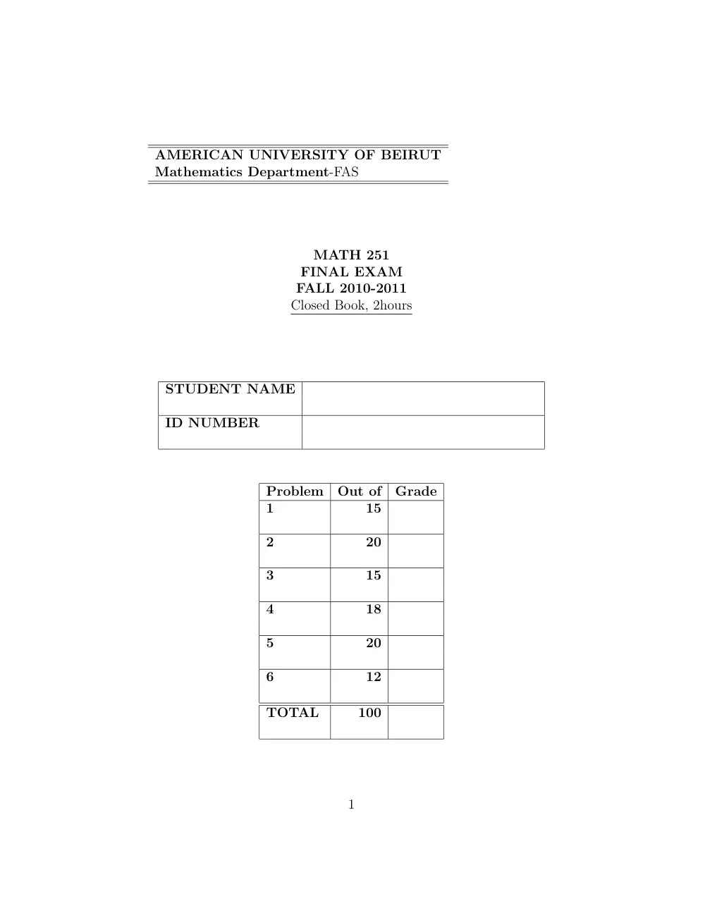
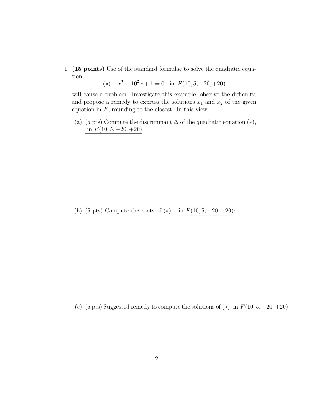
AMERICAN UNIVERSITY OF BEIRUT Mathematics Department-FAS MATH 251 FINAL EXAM FALL 2010-2011 Closed Book, 2hours STUDENT NAME ID NUMBER Problem Out of Grade 1 15 2 20 3 15 4 18 5 20 6 12 TOTAL 100 1 1. (15 points) Use of the standard formulae to solve the quadratic equa- tion (∗) x2 − 103x + 1 = 0 in F(10, 5, −20, +20) will cause a problem. Investigate this example, observe the difficulty, and propose a remedy to express the solutions x1 and x2 of the given equation in F, rounding to the closest. 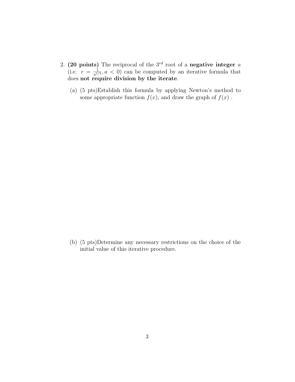In this view: (a) (5 pts) Compute the discriminant ∆ of the quadratic equation (∗), in F(10, 5, −20, +20): (b) (5 pts) Compute the roots of (∗) , in F(10, 5, −20, +20): (c) (5 pts) Suggested remedy to compute the solutions of (∗) in F(10, 5, −20, +20): 2 2. (20 points) The reciprocal of the 3rd root of a negative integer a (i.e. r = 1 a1/3, a < 0) can be computed by an iterative formula that does not require division by the iterate. (a) (5 pts)Establish this formula by applying Newton’s method to some appropriate function f(x), and draw the graph of f(x) . (b) (5 pts)Determine any necessary restrictions on the choice of the initial value of this iterative procedure. 3 (c) (5 pts)Prove that Newton’s method is Quadratic. (d) (5 pts)Prove that rn+1−r = (rn−r)2F(rn) where F is a quadratic polynomial in rn, to be determined. 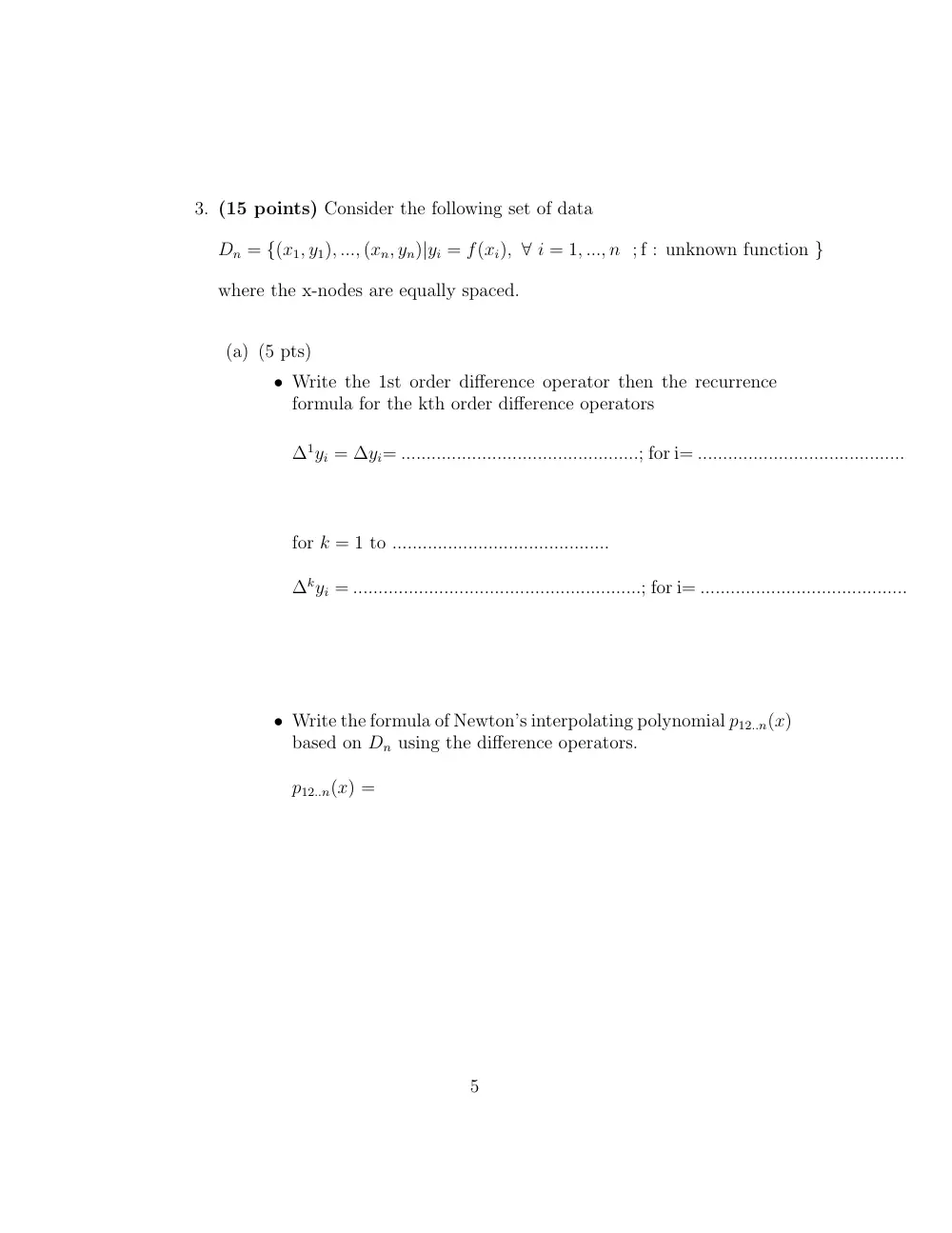4 3. (15 points) Consider the following set of data Dn = {(x1, y1), ..., (xn, yn)|yi = f(xi), ∀ i = 1, ..., n ; f : unknown function } where the x-nodes are equally spaced. (a) (5 pts) • Write the 1st order difference operator then the recurrence formula for the kth order difference operators ∆1yi = ∆yi= ...............................................; for i= ......................................... for k = 1 to ........................................... ∆kyi = .........................................................; for i= ......................................... • Write the formula of Newton’s interpolating polynomial p12..n(x) based on Dn using the difference operators. 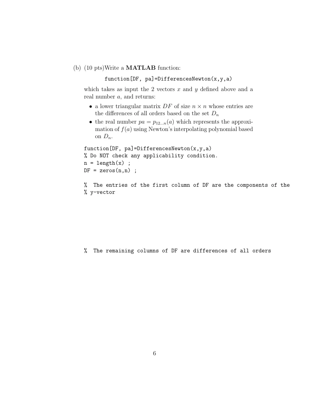p12..n(x) = 5 (b) (10 pts)Write a MATLAB function: function[DF, pa]=DifferencesNewton(x,y,a) which takes as input the 2 vectors x and y defined above and a real number a, and returns: • a lower triangular matrix DF of size n × n whose entries are the differences of all orders based on the set Dn • the real number pa = p12...n(a) which represents the approxi- mation of f(a) using Newton’s interpolating polynomial based on Dn. function[DF, pa]=DifferencesNewton(x,y,a) % Do NOT check any applicability condition. 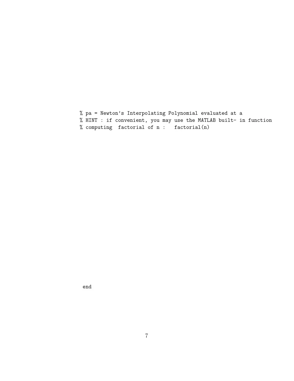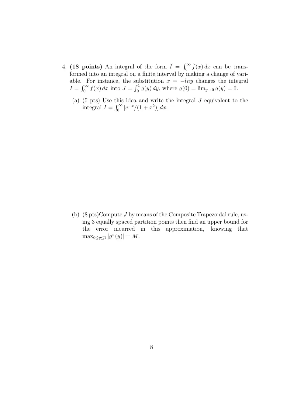n = length(x) ; DF = zeros(n,n) ; % The entries of the first column of DF are the components of the % y-vector % The remaining columns of DF are differences of all orders 6 % pa = Newton’s Interpolating Polynomial evaluated at a % HINT : if convenient, you may use the MATLAB built- in function % computing factorial of n : factorial(n) end 7 4. (18 points) An integral of the form I = � ∞ 0 f(x) dx can be trans- formed into an integral on a finite interval by making a change of vari- able. For instance, the substitution x = −lny changes the integral I = � ∞ 0 f(x) dx into J = � 1 0 g(y) dy, where g(0) = limy→0 g(y) = 0. (a) (5 pts) Use this idea and write the integral J equivalent to the integral I = � ∞ 0 [e−x/(1 + x2)] dx (b) (8 pts)Compute J by means of the Composite Trapezoidal rule, us- ing 3 equally spaced partition points then find an upper bound for the error incurred in this approximation, knowing that max0≤y≤1 |g”(y)| = M. 8 . 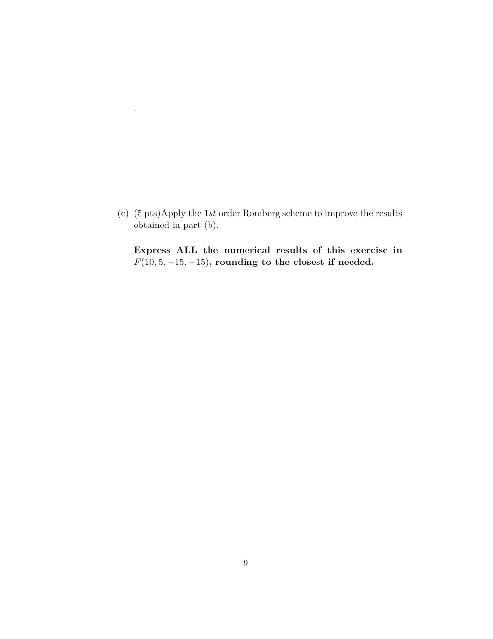(c) (5 pts)Apply the 1st order Romberg scheme to improve the results obtained in part (b). Express ALL the numerical results of this exercise in F(10, 5, −15, +15), rounding to the closest if needed. 9 5. (20 points) Let Dn = {(xi, yi)|i = 0, 1, ..., n = 2m, where yi = f(xi))} be a given set of data, where the x-coordinates are equally spaced, and where n is an even integer. (a) (5 pts)Based on the set Dn, prove that the 1st Romberg operator applied to the composite Trapezoid rule is equivalent to Simpson’s rule, that is prove that: R1(h) = S(h). (b) (5 pts)Derive the first 2 Romberg approximation formulae: S1(h) and S2(h) , applied to the Composite Simpson’s rule, given that: I = S(h) + s1h4 + s2h6 + ..... + sjh2j+2 + .... 10 (c) (10 pts)The next question deals with the following set of values for a function f(x), arranged in a table as follows: i xi f(xi) 0 0.000 1.0000 1 0.125 1.1108 2 0.250 1.1979 3 0.375 1.2663 4 0.500 1.3196 5 0.625 1.3600 6 0.750 1.3895 7 0.875 1.4093 8 1.000 1.4207 In order to approximate � 1 0 f(x) dx, based on Simpson’s rule and the formulae obtained in (a) and (b), fill in the empty slots of the following table adequately. Express all your results in F(10, 5, −15, +15). h T(h) S(h) S1(h) S2(h) h0 = 1 h0/2 = 0.5 h0/4 = 0.250 h0 8 = 0.1250 11 6. (12 points) Consider the following Initial value Problem: (IV P) � dy dt = t3 + y ; t ∈ [1, 2] y(1) = 3 To solve (IVP) in F(10, 4, −20, +20) (rounding to the closest): (a) (5 pts) (IVP) is first solved on [1, 1.5] using the discrete scheme of Euler’s method: (RK1). • Write first the formulae for this scheme: (RK1) � ................................................................ yi+1 = .................................................... • Use 2 steps ONLY of this scheme to approximate y(1.25) and y(1.50). i ti yi k1 yi+1 0 1.00 . . . 1 . . . . 2 . . . . 12 (b) (7 pts)(IVP) is then solved on [1.5,2] using the discrete scheme of the 2nd order Runge Kutta method - Midpoint Rule: (RK2.M). • Write then the formulae of this scheme: (RK2.M)    ............................................................... ................................................................ yi+1 = .................................................... • Use 2 steps ONLY of this scheme to approximate y(1.75) and y(2.00). i ti yi k1 k2 yi+1 0 1.50 . . . . 1 . . . . . 2 . . . . . 13