MATH 251 Final No Solution, Spring 2012

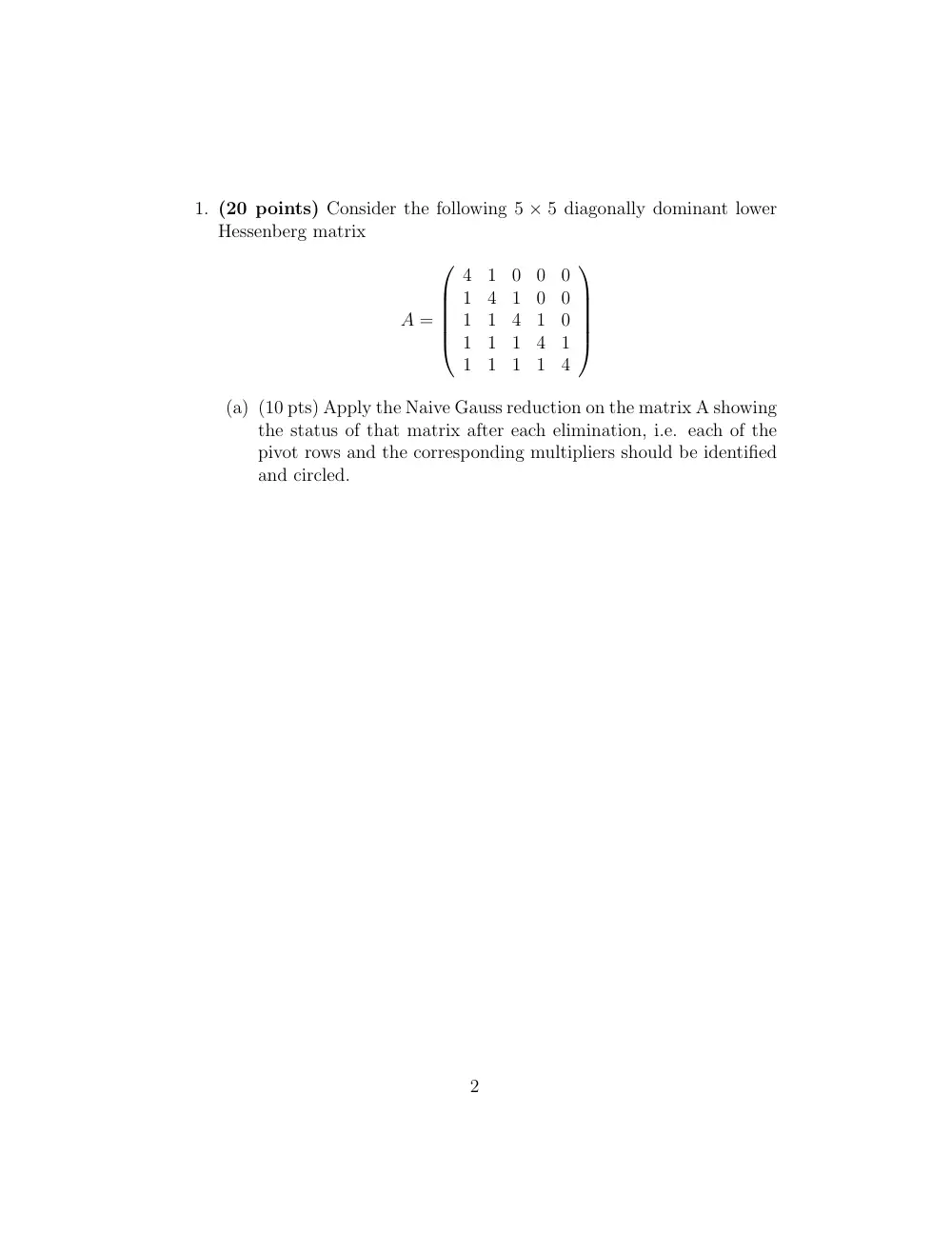
AMERICAN UNIVERSITY OF BEIRUT Mathematics Department-FAS MATH 251 FINAL EXAM SPRING 2011-2012 Closed Book, 2hours STUDENT NAME ID NUMBER Problem Out of Grade 1 20 2 20 3 20 4 16 5 24 TOTAL 100 1 1. (20 points) Consider the following 5 × 5 diagonally dominant lower Hessenberg matrix A =       4 1 0 0 0 1 4 1 0 0 1 1 4 1 0 1 1 1 4 1 1 1 1 1 4       (a) (10 pts) Apply the Naive Gauss reduction on the matrix A showing the status of that matrix after each elimination, i.e. each of the pivot rows and the corresponding multipliers should be identified and circled. 2 ... 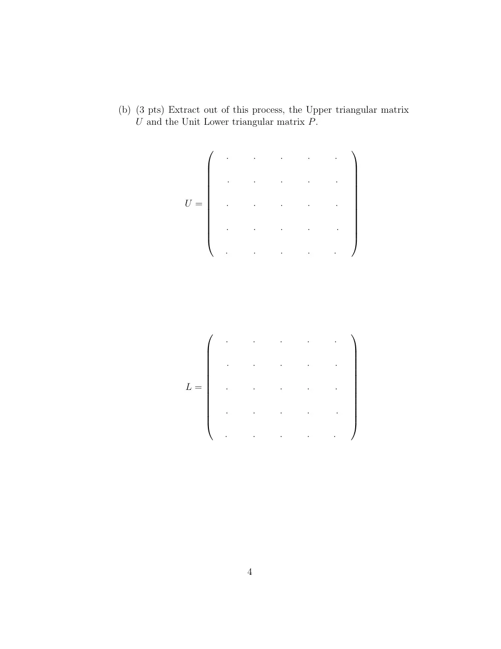3 (b) (3 pts) Extract out of this process, the Upper triangular matrix U and the Unit Lower triangular matrix P. U =               . . . . . . . . . . . . . . . . . . . . . . . . .               L =               . . . . . . . . . . . . . . . . . . . . . . . . . 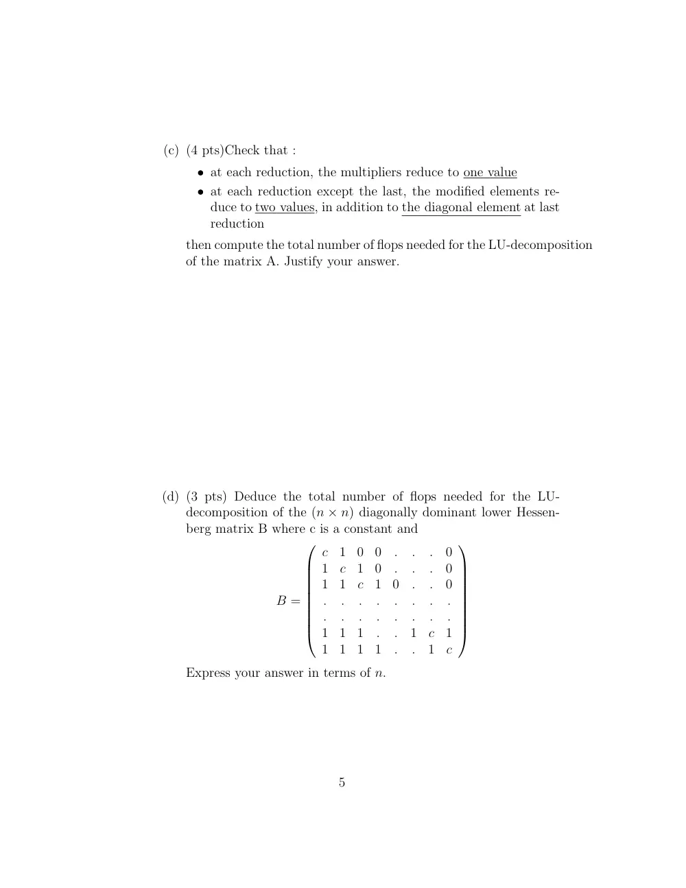              4 (c) (4 pts)Check that : • at each reduction, the multipliers reduce to one value • at each reduction except the last, the modified elements re- duce to two values, in addition to the diagonal element at last reduction then compute the total number of flops needed for the LU-decomposition of the matrix A. Justify your answer. (d) (3 pts) Deduce the total number of flops needed for the LU- decomposition of the (n × n) diagonally dominant lower Hessen- berg matrix B where c is a constant and B =           c 1 0 0 . . . 0 1 c 1 0 . . . 0 1 1 c 1 0 . . 0 . . . . . . . . . . . . . . . . 1 1 1 . . 1 c 1 1 1 1 1 . . 1 c           Express your answer in terms of n. 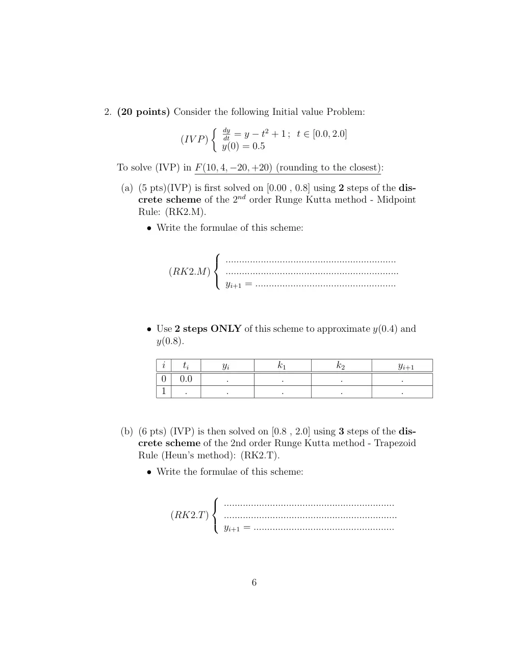5 2. (20 points) Consider the following Initial value Problem: (IV P) � dy dt = y − t2 + 1 ; t ∈ [0.0, 2.0] y(0) = 0.5 To solve (IVP) in F(10, 4, −20, +20) (rounding to the closest): (a) (5 pts)(IVP) is first solved on [0.00 , 0.8] using 2 steps of the dis- crete scheme of the 2nd order Runge Kutta method - Midpoint Rule: (RK2.M). • Write the formulae of this scheme: (RK2.M)    ............................................................... ................................................................ yi+1 = .................................................... • Use 2 steps ONLY of this scheme to approximate y(0.4) and y(0.8). i ti yi k1 k2 yi+1 0 0.0 . . . . 1 . . . . . (b) (6 pts) (IVP) is then solved on [0.8 , 2.0] using 3 steps of the dis- crete scheme of the 2nd order Runge Kutta method - Trapezoid Rule (Heun’s method): (RK2.T). • Write the formulae of this scheme: (RK2.T)    ............................................................... ................................................................ yi+1 = .................................................... 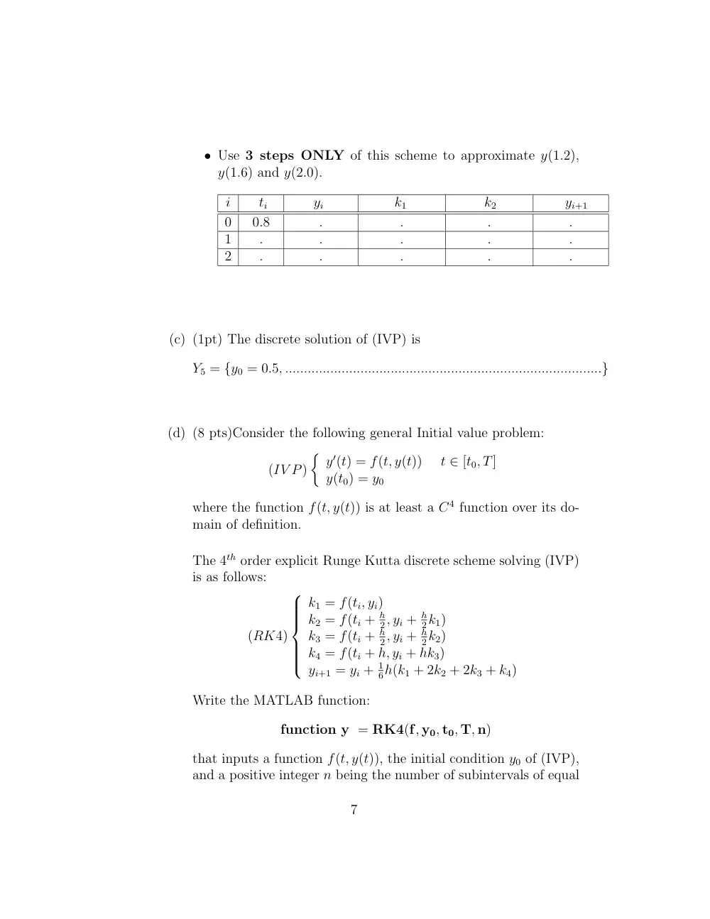6 • Use 3 steps ONLY of this scheme to approximate y(1.2), y(1.6) and y(2.0). i ti yi k1 k2 yi+1 0 0.8 . . . . 1 . . . . . 2 . . . . . (c) (1pt) The discrete solution of (IVP) is Y5 = {y0 = 0.5, ....................................................................................} (d) (8 pts)Consider the following general Initial value problem: (IV P) � y′(t) = f(t, y(t)) t ∈ [t0, T] y(t0) = y0 where the function f(t, y(t)) is at least a C4 function over its do- main of definition. The 4th order explicit Runge Kutta discrete scheme solving (IVP) is as follows: (RK4)            k1 = f(ti, yi) k2 = f(ti + h 2, yi + h 2k1) k3 = f(ti + h 2, yi + h 2k2) k4 = f(ti + h, yi + hk3) yi+1 = yi + 1 6h(k1 + 2k2 + 2k3 + k4) Write the MATLAB function: function y = RK4(f, y0, t0, T, n) that inputs a function f(t, y(t)), the initial condition y0 of (IVP), and a positive integer n being the number of subintervals of equal 7 length subdividing the time interval [t0, T]. This function outputs the discrete solution of (IVP) using the (RK4) discrete scheme as a vector y of length (n + 1). 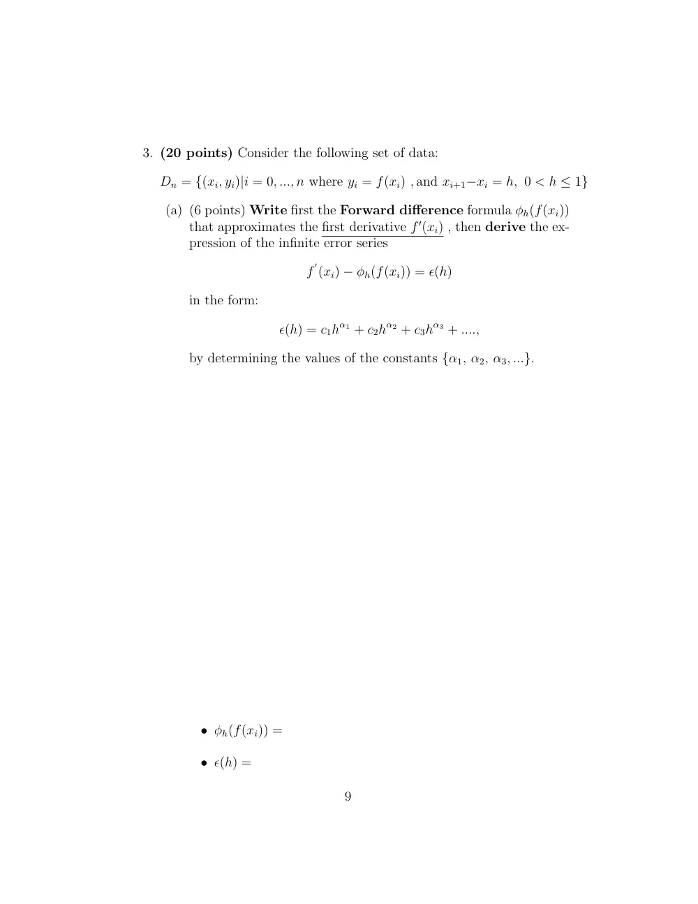function y = RK4(f, y0, t0, T, n) Compute the time step h 8 3. (20 points) Consider the following set of data: Dn = {(xi, yi)|i = 0, ..., n where yi = f(xi) , and xi+1−xi = h, 0 < h ≤ 1} (a) (6 points) Write first the Forward difference formula φh(f(xi)) that approximates the first derivative f ′(xi) , then derive the ex- pression of the infinite error series f ′(xi) − φh(f(xi)) = ϵ(h) in the form: ϵ(h) = c1hα1 + c2hα2 + c3hα3 + ...., by determining the values of the constants {α1, α2, α3, ...}. • φh(f(xi)) = • ϵ(h) = 9 (b) (6 points) Based on the Forward difference formula, derive Richard- son extrapolation operators of orders 1 and 2 and the order of their error series. • 1st order Richardson extrapolation operator: φ1 h(f(xi)) = Corresponding Error = O(...........) • 2nd order Richardson extrapolation operator: φ2 h(f(xi)) = Corresponding Error = O(...........) 10 (c) (8 pts) Let f(x) = x + ex. For the purpose of approximating f ′(1.0) and then improving this approximation, fill in the empty slots in the following table adequately, starting with h0 = 0.4. Express all the results obtained in F(10, 5, −15, +15). h φh(.) φ1 h(.) φ2 h(.) h0 = 0.4 h0/2 h0/4 Best approximation to f ′(1.0) : 11 4. (16 points)In order to approximate the double integral I = � 2 1.4 � 1.5 1 ln(x + 2y) dy dx over the rectangle R = {1 ≤ y ≤ 1.5 ; 1.4 ≤ x ≤ 2}, write first I as : I = � 2 1.4 [ � 1.5 1 ln(x + 2y) dy ] dx = � 2 1.4 J dx where J = � 1.5 1 ln(x + 2y) dy • In a first step, treating x as a constant, approximate J using the Composite Trapezoidal Rule, by partitioning the interval [1, 1.5] into to 2 subintervals of equal length. (Your answer should be expressed in terms of some function of x). J = � 1.5 1 ln(x + 2y) dy ≈ T(0.25) = g(x) = • Secondly, approximate I = � 2 1.4 J dx ≈ � 2 1.4 g(x) dx using the Composite Midpoint Rule, by partitioning the interval [1.4, 2] into to 2 subintervals of equal length. (Express your answer with a precision p = 4 rounding to the closest). I = � 2 1.4 J dx ≈ M(0.3) = 12 5. (24 points) Consider the function f(x) = x2 − a where a ≥ 1. (a) (7 pts)Plot the graph of f, then write Newton’s formula: rn+1 = g(rn) that computes the negative root of the function f. Is there any restriction on the initial condition r0? Justify your answer. (b) (7 pts)Use part (a) to compute − √ 3 up to 5 decimal figures rounding to the closest. (Locate the root first). 13 (c) (5 pts) Use the general case where f(x) = x2 − a, and the equa- tion derived in (a) to prove that: ∀n ≥ 0 , (rn+1 − r) < 0 (i.e. all the elements of the sequence {rn}n≥1 generated by New- ton’s method lie to the left of r) (Hint: Let a = r2) (d) (5 pts)Show that Newton’s iterative sequence {rn}n≥1 derived in (a) is an increasing sequence converging to r. For that purpose: • Prove that ∀n ≥ 1 , rn+1 − rn > 0 14 • Prove next that the sequence {rn} converges to r, i.e. that: lim n→∞ rn = r Hint: Use (c) and show first by induction on n that : r1 − r 2n < ... < rn−1 − r 22 < rn − r 21 < rn+1 − r < 0 15