MECH 420 Problems Chap 6, Fall 2012

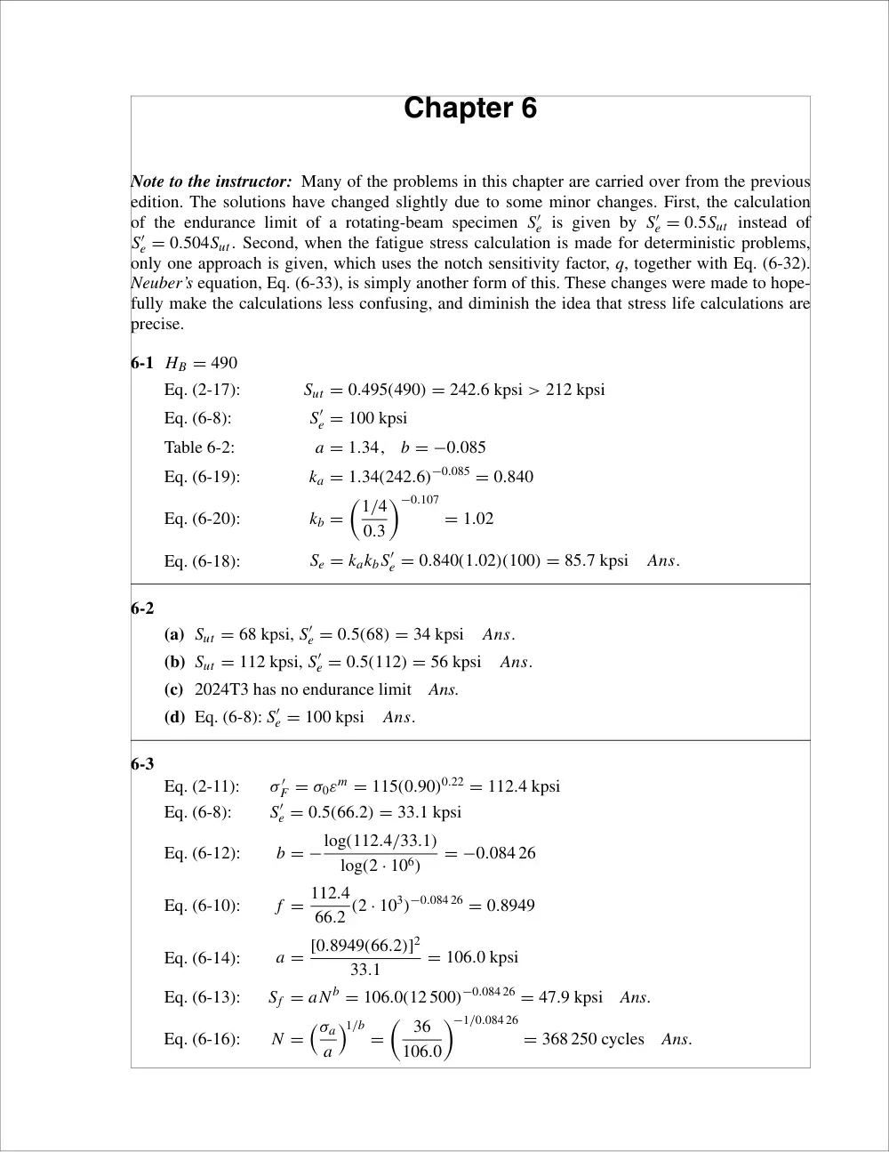
Chapter 6 Note to the instructor: Many of the problems in this chapter are carried over from the previous edition. The solutions have changed slightly due to some minor changes. First, the calculation of the endurance limit of a rotating-beam specimen S′ e is given by S′ e = 0.5Sut instead of S′ e = 0.504Sut. Second, when the fatigue stress calculation is made for deterministic problems, only one approach is given, which uses the notch sensitivity factor, q, together with Eq. (6-32). Neuber’s equation, Eq. (6-33), is simply another form of this. These changes were made to hope- fully make the calculations less confusing, and diminish the idea that stress life calculations are precise. 6-1 HB = 490 Eq. (2-17): Sut = 0.495(490) = 242.6 kpsi > 212 kpsi Eq. (6-8): S′ e = 100 kpsi Table 6-2: a = 1.34, b = −0.085 Eq. (6-19): ka = 1.34(242.6)−0.085 = 0.840 Eq. (6-20): kb = �1/4 0.3 �−0.107 = 1.02 Eq. (6-18): Se = kakbS′ e = 0.840(1.02)(100) = 85.7 kpsi Ans. 6-2 (a) Sut = 68 kpsi, S′ e = 0.5(68) = 34 kpsi Ans. (b) Sut = 112 kpsi, S′ e = 0.5(112) = 56 kpsi Ans. (c) 2024T3 has no endurance limit Ans. (d) Eq. (6-8): S′ e = 100 kpsi Ans. 6-3 Eq. (2-11): σ ′ F = σ0εm = 115(0.90)0.22 = 112.4 kpsi Eq. (6-8): S′ e = 0.5(66.2) = 33.1 kpsi Eq. (6-12): b = −log(112.4/33.1) log(2 · 106) = −0.084 26 Eq. (6-10): f = 112.4 66.2 (2 · 103)−0.084 26 = 0.8949 Eq. (6-14): a = [0.8949(66.2)]2 33.1 = 106.0 kpsi Eq. (6-13): Sf = aN b = 106.0(12 500)−0.084 26 = 47.9 kpsi Ans. Eq. (6-16): N = �σa a �1/b = � 36 106.0 �−1/0.084 26 = 368 250 cycles Ans. 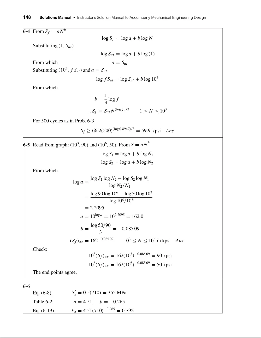148 Solutions Manual • Instructor’s Solution Manual to Accompany Mechanical Engineering Design 6-4 From Sf = aN b log Sf = log a + b log N Substituting (1, Sut) log Sut = log a + b log (1) From which a = Sut Substituting (103, f Sut) and a = Sut log f Sut = log Sut + b log 103 From which b = 1 3 log f ∴ Sf = Sut N (log f )/3 1 ≤ N ≤ 103 For 500 cycles as in Prob. 6-3 Sf ≥ 66.2(500)(log 0.8949)/3 = 59.9 kpsi Ans. 6-5 Read from graph: (103, 90) and (106, 50). From S = aN b log S1 = log a + b log N1 log S2 = log a + b log N2 From which log a = log S1 log N2 − log S2 log N1 log N2/N1 = log 90 log 106 − log 50 log 103 log 106/103 = 2.2095 a = 10log a = 102.2095 = 162.0 b = log 50/90 3 = −0.085 09 (Sf )ax = 162−0.085 09 103 ≤ N ≤ 106 in kpsi Ans. Check: 103(Sf )ax = 162(103)−0.085 09 = 90 kpsi 106(Sf )ax = 162(106)−0.085 09 = 50 kpsi The end points agree. 6-6 Eq. (6-8): S′ e = 0.5(710) = 355 MPa Table 6-2: a = 4.51, b = −0.265 Eq. 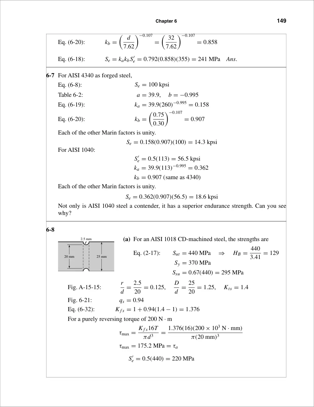(6-19): ka = 4.51(710)−0.265 = 0.792 Chapter 6 149 Eq. (6-20): kb = � d 7.62 �−0.107 = � 32 7.62 �−0.107 = 0.858 Eq. (6-18): Se = kakbS′ e = 0.792(0.858)(355) = 241 MPa Ans. 6-7 For AISI 4340 as forged steel, Eq. (6-8): Se = 100 kpsi Table 6-2: a = 39.9, b = −0.995 Eq. (6-19): ka = 39.9(260)−0.995 = 0.158 Eq. (6-20): kb = �0.75 0.30 �−0.107 = 0.907 Each of the other Marin factors is unity. Se = 0.158(0.907)(100) = 14.3 kpsi For AISI 1040: S′ e = 0.5(113) = 56.5 kpsi ka = 39.9(113)−0.995 = 0.362 kb = 0.907 (same as 4340) Each of the other Marin factors is unity. Se = 0.362(0.907)(56.5) = 18.6 kpsi Not only is AISI 1040 steel a contender, it has a superior endurance strength. Can you see why? 6-8 (a) For an AISI 1018 CD-machined steel, the strengths are Eq. (2-17): Sut = 440 MPa ⇒ HB = 440 3.41 = 129 Sy = 370 MPa Ssu = 0.67(440) = 295 MPa Fig. A-15-15: r d = 2.5 20 = 0.125, D d = 25 20 = 1.25, Kts = 1.4 Fig. 6-21: qs = 0.94 Eq. 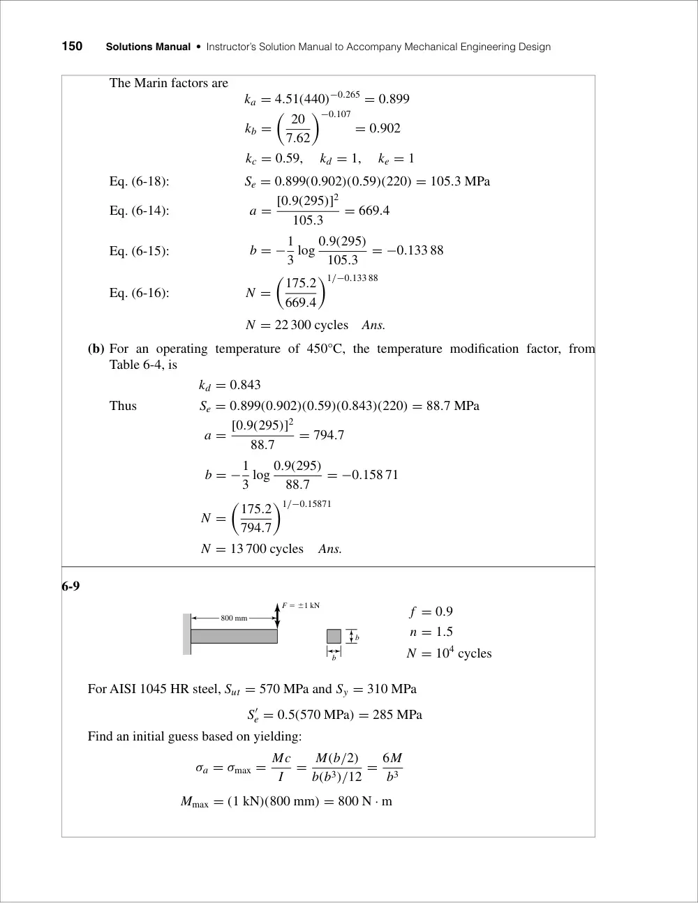(6-32): K f s = 1 + 0.94(1.4 − 1) = 1.376 For a purely reversing torque of 200 N · m τmax = K f s16T πd3 = 1.376(16)(200 × 103 N · mm) π(20 mm)3 τmax = 175.2 MPa = τa S′ e = 0.5(440) = 220 MPa 2.5 mm 20 mm 25 mm 150 Solutions Manual • Instructor’s Solution Manual to Accompany Mechanical Engineering Design The Marin factors are ka = 4.51(440)−0.265 = 0.899 kb = � 20 7.62 �−0.107 = 0.902 kc = 0.59, kd = 1, ke = 1 Eq. (6-18): Se = 0.899(0.902)(0.59)(220) = 105.3 MPa Eq. (6-14): a = [0.9(295)]2 105.3 = 669.4 Eq. (6-15): b = −1 3 log 0.9(295) 105.3 = −0.133 88 Eq. (6-16): N = �175.2 669.4 �1/−0.133 88 N = 22 300 cycles Ans. (b) For an operating temperature of 450°C, the temperature modification factor, from Table 6-4, is kd = 0.843 Thus Se = 0.899(0.902)(0.59)(0.843)(220) = 88.7 MPa a = [0.9(295)]2 88.7 = 794.7 b = −1 3 log 0.9(295) 88.7 = −0.158 71 N = �175.2 794.7 �1/−0.15871 N = 13 700 cycles Ans. 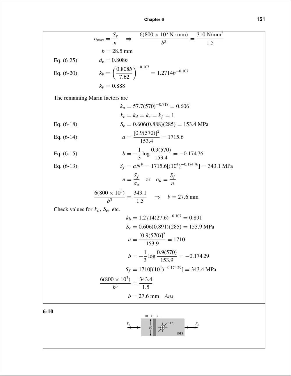6-9 f = 0.9 n = 1.5 N = 104 cycles For AISI 1045 HR steel, Sut = 570 MPa and Sy = 310 MPa S′ e = 0.5(570 MPa) = 285 MPa Find an initial guess based on yielding: σa = σmax = Mc I = M(b/2) b(b3)/12 = 6M b3 Mmax = (1 kN)(800 mm) = 800 N · m F � �1 kN b b 800 mm Chapter 6 151 σmax = Sy n ⇒ 6(800 × 103 N · mm) b3 = 310 N/mm2 1.5 b = 28.5 mm Eq. (6-25): de = 0.808b Eq. (6-20): kb = �0.808b 7.62 �−0.107 = 1.2714b−0.107 kb = 0.888 The remaining Marin factors are ka = 57.7(570)−0.718 = 0.606 kc = kd = ke = kf = 1 Eq. (6-18): Se = 0.606(0.888)(285) = 153.4 MPa Eq. (6-14): a = [0.9(570)]2 153.4 = 1715.6 Eq. (6-15): b = −1 3 log 0.9(570) 153.4 = −0.174 76 Eq. (6-13): Sf = aN b = 1715.6[(104)−0.174 76] = 343.1 MPa n = Sf σa or σa = Sf n 6(800 × 103) b3 = 343.1 1.5 ⇒ b = 27.6 mm Check values for kb, Se, etc. kb = 1.2714(27.6)−0.107 = 0.891 Se = 0.606(0.891)(285) = 153.9 MPa a = [0.9(570)]2 153.9 = 1710 b = −1 3 log 0.9(570) 153.9 = −0.174 29 Sf = 1710[(104)−0.174 29] = 343.4 MPa 6(800 × 103) b3 = 343.4 1.5 b = 27.6 mm Ans. 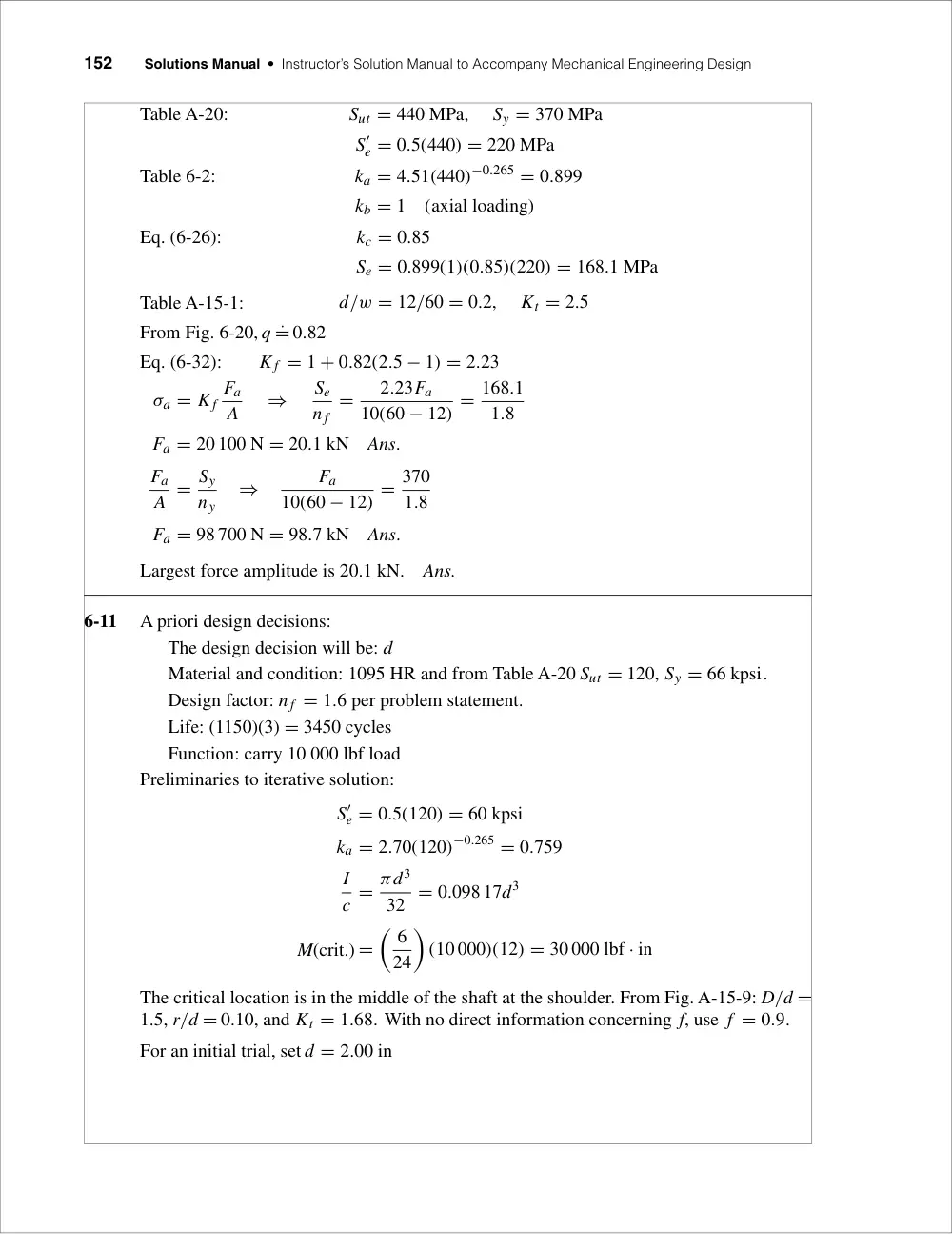6-10 12 Fa Fa 10 60 1018 152 Solutions Manual • Instructor’s Solution Manual to Accompany Mechanical Engineering Design Table A-20: Sut = 440 MPa, Sy = 370 MPa S′ e = 0.5(440) = 220 MPa Table 6-2: ka = 4.51(440)−0.265 = 0.899 kb = 1 (axial loading) Eq. (6-26): kc = 0.85 Se = 0.899(1)(0.85)(220) = 168.1 MPa Table A-15-1: d/w = 12/60 = 0.2, Kt = 2.5 From Fig. 6-20, q ˙= 0.82 Eq. (6-32): K f = 1 + 0.82(2.5 − 1) = 2.23 σa = K f Fa A ⇒ Se n f = 2.23Fa 10(60 − 12) = 168.1 1.8 Fa = 20 100 N = 20.1 kN Ans. Fa A = Sy ny ⇒ Fa 10(60 − 12) = 370 1.8 Fa = 98 700 N = 98.7 kN Ans. Largest force amplitude is 20.1 kN. Ans. 6-11 A priori design decisions: The design decision will be: d Material and condition: 1095 HR and from Table A-20 Sut = 120, Sy = 66 kpsi. Design factor: n f = 1.6 per problem statement. Life: (1150)(3) = 3450 cycles Function: carry 10 000 lbf load Preliminaries to iterative solution: S′ e = 0.5(120) = 60 kpsi ka = 2.70(120)−0.265 = 0.759 I c = πd3 32 = 0.098 17d3 M(crit.) = � 6 24 � (10 000)(12) = 30 000 lbf · in The critical location is in the middle of the shaft at the shoulder. From Fig. A-15-9: D/d = 1.5, r/d = 0.10, and Kt = 1.68. With no direct information concerning f, use f = 0.9. 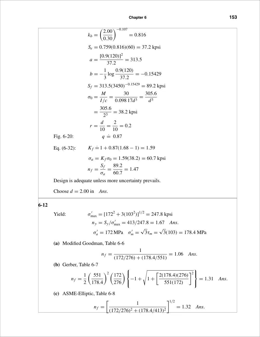For an initial trial, set d = 2.00 in Chapter 6 153 kb = �2.00 0.30 �−0.107 = 0.816 Se = 0.759(0.816)(60) = 37.2 kpsi a = [0.9(120)]2 37.2 = 313.5 b = −1 3 log 0.9(120) 37.2 = −0.15429 Sf = 313.5(3450)−0.15429 = 89.2 kpsi σ0 = M I/c = 30 0.098 17d3 = 305.6 d3 = 305.6 23 = 38.2 kpsi r = d 10 = 2 10 = 0.2 Fig. 6-20: q ˙= 0.87 Eq. (6-32): K f ˙= 1 + 0.87(1.68 − 1) = 1.59 σa = K f σ0 = 1.59(38.2) = 60.7 kpsi n f = Sf σa = 89.2 60.7 = 1.47 Design is adequate unless more uncertainty prevails. Choose d = 2.00 in Ans. 6-12 Yield: σ ′ max = [1722 + 3(1032)]1/2 = 247.8 kpsi ny = Sy/σ ′ max = 413/247.8 = 1.67 Ans. σ ′ a = 172 MPa σ ′ m = √ 3τm = √ 3(103) = 178.4 MPa (a) Modified Goodman, Table 6-6 n f = 1 (172/276) + (178.4/551) = 1.06 Ans. (b) Gerber, Table 6-7 n f = 1 2 � 551 178.4 �2 �172 276 �   −1 + � 1 + �2(178.4)(276) 551(172) �2    = 1.31 Ans. (c) ASME-Elliptic, Table 6-8 n f = � 1 (172/276)2 + (178.4/413)2 �1/2 = 1.32 Ans. 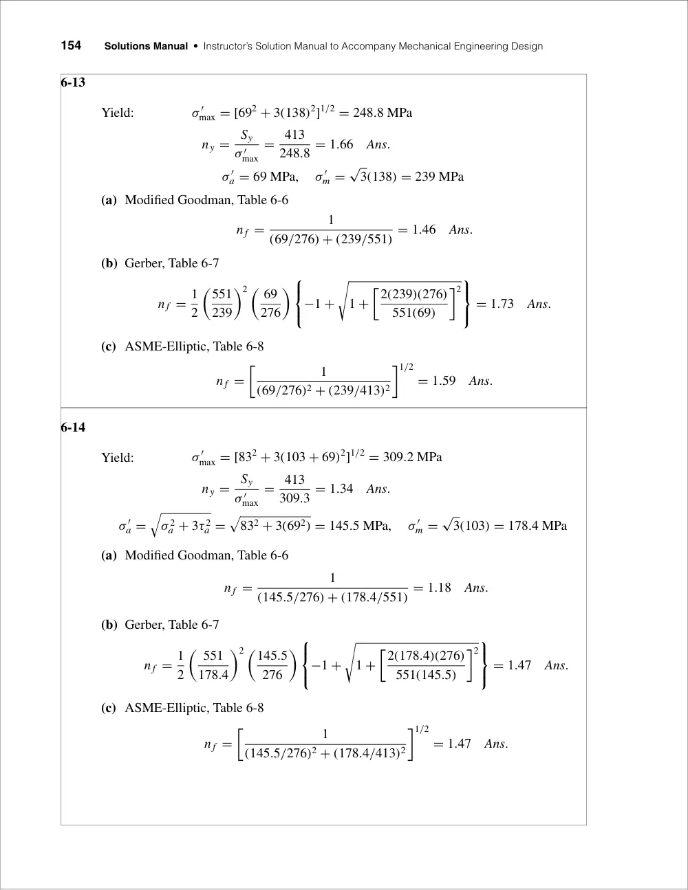154 Solutions Manual • Instructor’s Solution Manual to Accompany Mechanical Engineering Design 6-13 Yield: σ ′ max = [692 + 3(138)2]1/2 = 248.8 MPa ny = Sy σ ′max = 413 248.8 = 1.66 Ans. σ ′ a = 69 MPa, σ ′ m = √ 3(138) = 239 MPa (a) Modified Goodman, Table 6-6 n f = 1 (69/276) + (239/551) = 1.46 Ans. (b) Gerber, Table 6-7 n f = 1 2 �551 239 �2 � 69 276 �   −1 + � 1 + �2(239)(276) 551(69) �2    = 1.73 Ans. (c) ASME-Elliptic, Table 6-8 n f = � 1 (69/276)2 + (239/413)2 �1/2 = 1.59 Ans. 6-14 Yield: σ ′ max = [832 + 3(103 + 69)2]1/2 = 309.2 MPa ny = Sy σ ′max = 413 309.3 = 1.34 Ans. σ ′ a = � σ 2a + 3τ 2a = � 832 + 3(692) = 145.5 MPa, σ ′ m = √ 3(103) = 178.4 MPa (a) Modified Goodman, Table 6-6 n f = 1 (145.5/276) + (178.4/551) = 1.18 Ans. (b) Gerber, Table 6-7 n f = 1 2 � 551 178.4 �2 �145.5 276 �   −1 + � 1 + �2(178.4)(276) 551(145.5) �2    = 1.47 Ans. (c) ASME-Elliptic, Table 6-8 n f = � 1 (145.5/276)2 + (178.4/413)2 �1/2 = 1.47 Ans. 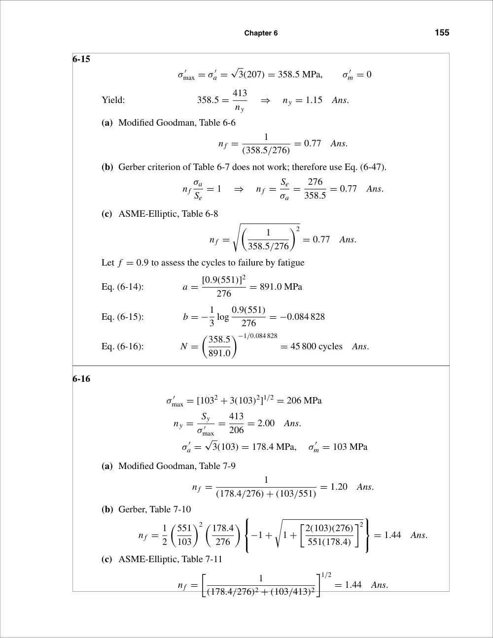Chapter 6 155 6-15 σ ′ max = σ ′ a = √ 3(207) = 358.5 MPa, σ ′ m = 0 Yield: 358.5 = 413 ny ⇒ ny = 1.15 Ans. (a) Modified Goodman, Table 6-6 n f = 1 (358.5/276) = 0.77 Ans. (b) Gerber criterion of Table 6-7 does not work; therefore use Eq. (6-47). n f σa Se = 1 ⇒ n f = Se σa = 276 358.5 = 0.77 Ans. (c) ASME-Elliptic, Table 6-8 n f = �� 1 358.5/276 �2 = 0.77 Ans. Let f = 0.9 to assess the cycles to failure by fatigue Eq. (6-14): a = [0.9(551)]2 276 = 891.0 MPa Eq. (6-15): b = −1 3 log 0.9(551) 276 = −0.084 828 Eq. (6-16): N = �358.5 891.0 �−1/0.084 828 = 45 800 cycles Ans. 6-16 σ ′ max = [1032 + 3(103)2]1/2 = 206 MPa ny = Sy σ ′max = 413 206 = 2.00 Ans. σ ′ a = √ 3(103) = 178.4 MPa, σ ′ m = 103 MPa (a) Modified Goodman, Table 7-9 n f = 1 (178.4/276) + (103/551) = 1.20 Ans. (b) Gerber, Table 7-10 n f = 1 2 �551 103 �2 �178.4 276 �   −1 + � 1 + �2(103)(276) 551(178.4) �2    = 1.44 Ans. (c) ASME-Elliptic, Table 7-11 n f = � 1 (178.4/276)2 + (103/413)2 �1/2 = 1.44 Ans. 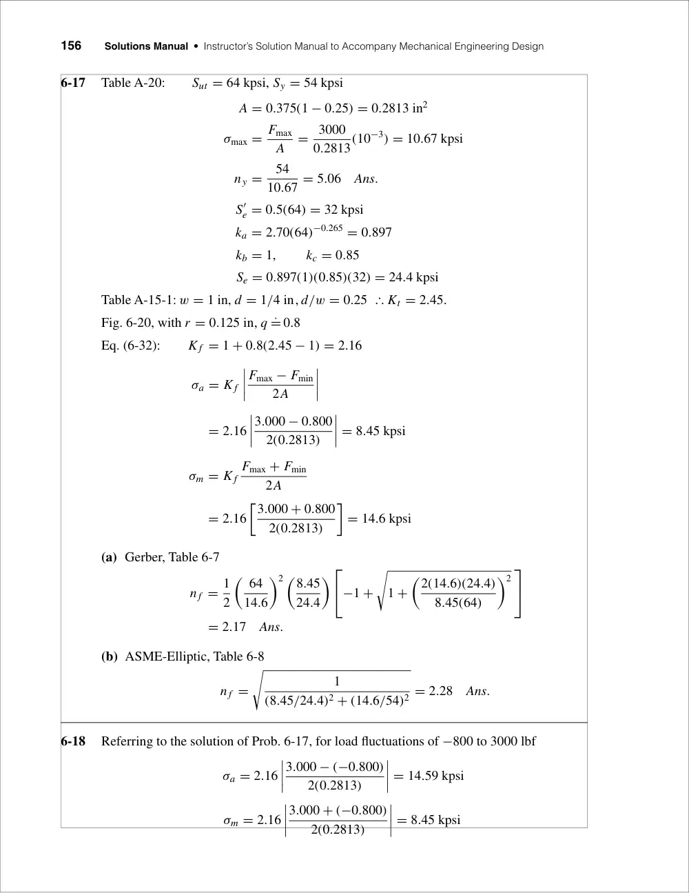156 Solutions Manual • Instructor’s Solution Manual to Accompany Mechanical Engineering Design 6-17 Table A-20: Sut = 64 kpsi, Sy = 54 kpsi A = 0.375(1 − 0.25) = 0.2813 in2 σmax = Fmax A = 3000 0.2813(10−3) = 10.67 kpsi ny = 54 10.67 = 5.06 Ans. S′ e = 0.5(64) = 32 kpsi ka = 2.70(64)−0.265 = 0.897 kb = 1, kc = 0.85 Se = 0.897(1)(0.85)(32) = 24.4 kpsi Table A-15-1: w = 1 in, d = 1/4 in, d/w = 0.25 � Kt = 2.45. Fig. 6-20, with r = 0.125 in, q ˙= 0.8 Eq. (6-32): K f = 1 + 0.8(2.45 − 1) = 2.16 σa = K f ���� Fmax − Fmin 2A ���� = 2.16 ���� 3.000 − 0.800 2(0.2813) ���� = 8.45 kpsi σm = K f Fmax + Fmin 2A = 2.16 �3.000 + 0.800 2(0.2813) � = 14.6 kpsi (a) Gerber, Table 6-7 n f = 1 2 � 64 14.6 �2 �8.45 24.4 �  −1 + � 1 + �2(14.6)(24.4) 8.45(64) �2   = 2.17 Ans. (b) ASME-Elliptic, Table 6-8 n f = � 1 (8.45/24.4)2 + (14.6/54)2 = 2.28 Ans. 6-18 Referring to the solution of Prob. 6-17, for load fluctuations of −800 to 3000 lbf σa = 2.16 ���� 3.000 − (−0.800) 2(0.2813) ���� = 14.59 kpsi σm = 2.16 ���� 3.000 + (−0.800) 2(0.2813) ���� = 8.45 kpsi Chapter 6 157 (a) Table 6-7, DE-Gerber n f = 1 2 � 64 8.45 �2 �14.59 24.4 � −1 + � 1 + �2(8.45)(24.4) 64(14.59) �2   = 1.60 Ans. (b) Table 6-8, DE-Elliptic n f = � 1 (14.59/24.4)2 + (8.45/54)2 = 1.62 Ans. 6-19 Referring to the solution of Prob. 6-17, for load fluctuations of 800 to −3000 lbf σa = 2.16 ���� 0.800 − (−3.000) 2(0.2813) ���� = 14.59 kpsi σm = 2.16 �0.800 + (−3.000) 2(0.2813) � = −8.45 kpsi (a) We have a compressive midrange stress for which the failure locus is horizontal at the Se level. n f = Se σa = 24.4 14.59 = 1.67 Ans. (b) Same as (a) n f = Se σa = 24.4 14.59 = 1.67 Ans. 6-20 Sut = 0.495(380) = 188.1 kpsi S′ e = 0.5(188.1) = 94.05 kpsi ka = 14.4(188.1)−0.718 = 0.335 For a non-rotating round bar in bending, Eq. (6-24) gives: de = 0.370d = 0.370(3/8) = 0.1388 in kb = �0.1388 0.3 �−0.107 = 1.086 Se = 0.335(1.086)(94.05) = 34.22 kpsi Fa = 30 − 15 2 = 7.5 lbf, Fm = 30 + 15 2 = 22.5 lbf σm = 32Mm πd3 = 32(22.5)(16) π(0.3753) (10−3) = 69.54 kpsi 158 Solutions Manual • Instructor’s Solution Manual to Accompany Mechanical Engineering Design σa = 32(7.5)(16) π(0.3753) (10−3) = 23.18 kpsi r = 23.18 69.54 = 0.333 0 (a) Modified Goodman, Table 6-6 n f = 1 (23.18/34.22) + (69.54/188.1) = 0.955 Since finite failure is predicted, proceed to calculate N From Fig. 6-18, for Sut = 188.1 kpsi, f = 0.778 Eq. (6-14): a = [0.7781(188.1)]2 34.22 = 625.8 kpsi Eq. (6-15): b = −1 3 log 0.778(188.1) 34.22 = −0.210 36 σa Sf + σm Sut = 1 ⇒ Sf = σa 1 − (σm/Sut) = 23.18 1 − (69.54/188.1) = 36.78 kpsi Eq. (7-15) with σa = Sf N = �36.78 625.8 �1/−0.210 36 = 710 000 cycles Ans. (b) Gerber, Table 6-7 n f = 1 2 �188.1 69.54 �2 �23.18 34.22 �   −1 + � 1 + �2(69.54)(34.22) 188.1(23.18) �2    = 1.20 Thus, infinite life is predicted (N ≥ 106 cycles). Ans. 6-21 (a) I = 1 12(18)(33) = 40.5 mm4 y = Fl3 3E I ⇒ F = 3E I y l3 Fmin = 3(207)(109)(40.5)(10−12)(2)(10−3) (1003)(10−9) = 50.3 N Ans. Fmax = 6 2(50.3) = 150.9 N Ans. (b) M = 0.1015F N · m A = 3(18) = 54 mm2 F F M 101.5 mm Chapter 6 159 Curved beam: rn = h ln(ro/ri) = 3 ln(6/3) = 4.3281 mm rc = 4.5 mm, e = rc − rn = 4.5 − 4.3281 = 0.1719 mm σi = − Mci Aeri − F A = −(0.1015F)(1.5 − 0.1719) 54(0.1719)(3)(10−3) − F 54 = −4.859F MPa σo = Mco Aero − F A = (0.1015F)(1.5 + 0.1719) 54(0.1719)(6)(10−3) − F 54 = 3.028F MPa (σi)min = −4.859(150.9) = −733.2 MPa (σi)max = −4.859(50.3) = −244.4 MPa (σo)max = 3.028(150.9) = 456.9 MPa (σo)min = 3.028(50.3) = 152.3 MPa Eq. (2-17) Sut = 3.41(490) = 1671 MPa Per the problem statement, estimate the yield as Sy = 0.9Sut = 0.9(1671) = 1504 MPa. Then from Eq. (6-8), S′ e = 700 MPa; Eq. (6-19), ka = 1.58(1671)−0.085 = 0.841; Eq. (6-25) de = 0.808[18(3)]1/2 = 5.938 mm; and Eq. (6-20), kb = (5.938/7.62)−0.107 = 1.027. Se = 0.841(1.027)(700) = 605 MPa At Inner Radius (σi)a = ���� −733.2 + 244.4 2 ���� = 244.4 MPa (σi)m = −733.2 − 244.4 2 = −488.8 MPa Load line: σm = −244.4 − σa Langer (yield) line: σm = σa − 1504 = −244.4 − σa Intersection: σa = 629.8 MPa, σm = −874.2 MPa (Note that σa is more than 605 MPa) Yield: ny = 629.8 244.4 = 2.58 244.4 488.4 �m �a �1504 605 1504 MPa 160 Solutions Manual • Instructor’s Solution Manual to Accompany Mechanical Engineering Design Fatigue: n f = 605 244.4 = 2.48 Thus, the spring is likely to fail in fatigue at the inner radius. Ans. At Outer Radius (σo)a = 456.9 − 152.3 2 = 152.3 MPa (σo)m = 456.9 + 152.3 2 = 304.6 MPa Yield load line: σm = 152.3 + σa Langer line: σm = 1504 − σa = 152.3 + σa Intersection: σa = 675.9 MPa, σm = 828.2 MPa ny = 675.9 152.3 = 4.44 Fatigue line: σa = [1 − (σm/Sut)2]Se = σm − 152.3 605 � 1 − � σm 1671 �2� = σm − 152.3 σ 2 m + 4615.3σm − 3.4951(106) = 0 σm = −4615.3 + � 4615.32 + 4(3.4951)(106) 2 = 662.2 MPa σa = 662.2 − 152.3 = 509.9 MPa n f = 509.9 152.3 = 3.35 Thus, the spring is not likely to fail in fatigue at the outer radius. Ans. 6-22 The solution at the inner radius is the same as in Prob. 6-21. At the outer radius, the yield solution is the same. Fatigue line: σa = � 1 − σm Sut � Se = σm − 152.3 605 � 1 − σm 1671 � = σm − 152.3 1.362σm = 757.3 ⇒ σm = 556.0 MPa σa = 556.0 − 152.3 = 403.7 MPa n f = 403.7 152.3 = 2.65 Ans. Chapter 6 161 6-23 Preliminaries: Table A-20: Sut = 64 kpsi, Sy = 54 kpsi S′ e = 0.5(64) = 32 kpsi ka = 2.70(64)−0.265 = 0.897 kb = 1 kc = 0.85 Se = 0.897(1)(0.85)(32) = 24.4 kpsi Fillet: Fig. A-15-5: D = 3.75 in, d = 2.5 in, D/d = 3.75/2.5 = 1.5, and r/d = 0.25/2.5 = 0.10 ∴ Kt = 2.1. Fig. 6-20 with r � 0.25 in, q ˙= 0.82 Eq. (6-32): K f = 1 + 0.82(2.1 − 1) = 1.90 σmax = 4 2.5(0.5) = 3.2 kpsi σmin = −16 2.5(0.5) = −12.8 kpsi σa = 1.90 ���� 3.2 − (−12.8) 2 ���� = 15.2 kpsi σm = 1.90 �3.2 + (−12.8) 2 � = −9.12 kpsi ny = ���� Sy σmin ���� = ���� 54 −12.8 ���� = 4.22 Since the midrange stress is negative, Sa = Se = 24.4 kpsi n f = Sa σa = 24.4 15.2 = 1.61 Hole: Fig. A-15-1: d/w = 0.75/3.75 = 0.20, Kt = 2.5. Fig. 6-20, with r � 0.375 in, q ˙= 0.85 Eq. (6-32): K f = 1 + 0.85(2.5 − 1) = 2.28 σmax = 4 0.5(3.75 − 0.75) = 2.67 kpsi σmin = −16 0.5(3.75 − 0.75) = −10.67 kpsi σa = 2.28 ���� 2.67 − (−10.67) 2 ���� = 15.2 kpsi σm = 2.28 2.67 + (−10.67) 2 = −9.12 kpsi 162 Solutions Manual • Instructor’s Solution Manual to Accompany Mechanical Engineering Design Since the midrange stress is negative, ny = ���� Sy σmin ���� = ���� 54 −10.67 ���� = 5.06 Sa = Se = 24.4 kpsi n f = Sa σa = 24.4 15.2 = 1.61 Thus the design is controlled by the threat of fatigue equally at the fillet and the hole; the minimum factor of safety is n f = 1.61. Ans. 6-24 (a) Curved beam in pure bending where M = −T throughout. The maximum stress will occur at the inner fiber where rc = 20 mm, but will be com- pressive. The maximum tensile stress will occur at the outer fiber where rc = 60 mm. Why? Inner fiber where rc = 20 mm rn = h ln(ro/ri) = 5 ln (22.5/17.5) = 19.8954 mm e = 20 − 19.8954 = 0.1046 mm ci = 19.8954 − 17.5 = 2.395 mm A = 25 mm2 σi = Mci Aeri = −T(2.395)10−3 25(10−6)0.1046(10−3)17.5(10−3)(10−6) = −52.34 T (1) where T is in N . m, and σi is in MPa. σm = 1 2(−52.34T) = −26.17T, σa = 26.17T For the endurance limit, S′ e = 0.5(770) = 385 MPa ka = 4.51(770)−0.265 = 0.775 de = 0.808[5(5)]1/2 = 4.04 mm kb = (4.04/7.62)−0.107 = 1.07 Se = 0.775(1.07)385 = 319.3 MPa For a compressive midrange component, σa = Se/n f . Thus, 26.17T = 319.3/3 ⇒ T = 4.07 N · m T T Chapter 6 163 Outer fiber where rc = 60 mm rn = 5 ln(62.5/57.5) = 59.96526 mm e = 60 − 59.96526 = 0.03474 mm co = 62.5 − 59.96526 = 2.535 mm σo = − Mci Aeri = − −T(2.535)10−3 25(10−6)0.03474(10−3)62.5(10−3)(10−6) = 46.7 T Comparing this with Eq. (1), we see that it is less in magnitude, but the midrange compo- nent is tension. σa = σm = 1 2(46.7T) = 23.35T Using Eq. (6-46), for modified Goodman, we have 23.35T 319.3 + 23.35T 770 = 1 3 ⇒ T = 3.22 N · m Ans. (b) Gerber, Eq. (6-47), at the outer fiber, 3(23.35T) 319.3 + �3(23.35T) 770 �2 = 1 reduces to T 2 + 26.51T − 120.83 = 0 T = 1 2 � −26.51 + � 26.512 + 4(120.83) � = 3.96 N · m Ans. (c) To guard against yield, use T of part (b) and the inner stress. ny = 420 52.34(3.96) = 2.03 Ans. 6-25 From Prob. 6-24, Se = 319.3 MPa, Sy = 420 MPa, and Sut = 770 MPa (a) Assuming the beam is straight, σmax = 6M bh2 = 6T 53[(10−3)3] = 48(106)T Goodman: 24T 319.3 + 24T 770 = 1 3 ⇒ T = 3.13 N · m Ans. (b) Gerber: 3(24)T 319.3 + �3(24)T 770 �2 = 1 T 2 + 25.79T − 114.37 = 1 T = 1 2 � −25.79 + � 25.792 + 4(114.37) � = 3.86 N · m Ans. 164 Solutions Manual • Instructor’s Solution Manual to Accompany Mechanical Engineering Design (c) Using σmax = 52.34(106)T from Prob. 6-24, ny = 420 52.34(3.86) = 2.08 Ans. 6-26 (a) τmax = 16K f sTmax πd3 Fig. 6-21 for HB > 200, r = 3 mm, qs .= 1 K f s = 1 + qs(Kts − 1) K f s = 1 + 1(1.6 − 1) = 1.6 Tmax = 2000(0.05) = 100 N · m, Tmin = 500 2000(100) = 25 N · m τmax = 16(1.6)(100)(10−6) π(0.02)3 = 101.9 MPa τmin = 500 2000(101.9) = 25.46 MPa τm = 1 2(101.9 + 25.46) = 63.68 MPa τa = 1 2(101.9 − 25.46) = 38.22 MPa Ssu = 0.67Sut = 0.67(320) = 214.4 MPa Ssy = 0.577Sy = 0.577(180) = 103.9 MPa S′ e = 0.5(320) = 160 MPa ka = 57.7(320)−0.718 = 0.917 de = 0.370(20) = 7.4 mm kb = � 7.4 7.62 �−0.107 = 1.003 kc = 0.59 Se = 0.917(1.003)(0.59)(160) = 86.8 MPa Modified Goodman, Table 6-6 n f = 1 (τa/Se) + (τm/Ssu) = 1 (38.22/86.8) + (63.68/214.4) = 1.36 Ans. (b) Gerber, Table 6-7 n f = 1 2 �Ssu τm �2 τa Se  −1 + � 1 + �2τmSe Ssuτa �2   = 1 2 �214.4 63.68 �2 38.22 86.8   −1 + � 1 + �2(63.68)(86.8) 214.4(38.22) �2    = 1.70 Ans. Chapter 6 165 6-27 Sy = 800 MPa, Sut = 1000 MPa (a) From Fig. 6-20, for a notch radius of 3 mm and Sut = 1 GPa, q .= 0.92. K f = 1 + q(Kt − 1) = 1 + 0.92(3 − 1) = 2.84 σmax = −K f 4P πd2 = − 2.84(4)P π(0.030)2 = −4018P σm = −σa = 1 2(−4018P) = −2009P T = f P � D + d 4 � Tmax = 0.3P �0.150 + 0.03 4 � = 0.0135P From Fig. 6-21, qs .= 0.95. Also, Kts is given as 1.8. Thus, K f s = 1 + qs(Kts − 1) = 1 + 0.95(1.8 − 1) = 1.76 τmax = 16K f sT πd3 = 16(1.76)(0.0135P) π(0.03)3 = 4482P τa = τm = 1 2(4482P) = 2241P Eqs. (6-55) and (6-56): σ ′ a = σ ′ m = � (σa/0.85)2 + 3τ 2 a �1/2 = � (−2009P/0.85)2 + 3(2241P)2�1/2 = 4545P S′ e = 0.5(1000) = 500 MPa ka = 4.51(1000)−0.265 = 0.723 kb = � 30 7.62 �−0.107 = 0.864 Se = 0.723(0.864)(500) = 312.3 MPa Modified Goodman: σ ′ a Se + σ ′ m Sut = 1 n 4545P 312.3(106) + 4545P 1000(106) = 1 3 ⇒ P = 17.5(103) N = 16.1 kN Ans. Yield (conservative): ny = Sy σ ′a + σ ′m ny = 800(106) 2(4545)(17.5)(103) = 5.03 Ans. (actual): σ ′ max = � σ 2 max + 3τ 2 max �1/2 = � (−4018P)2 + 3(4482P)2�1/2 = 8741P ny = Sy σ ′max = 800(106) 8741(17.5)103 = 5.22 166 Solutions Manual • Instructor’s Solution Manual to Accompany Mechanical Engineering Design (b) If the shaft is not rotating, τm = τa = 0. σm = σa = −2009P kb = 1 (axial) kc = 0.85 (Since there is no tension, kc = 1 might be more appropriate.) Se = 0.723(1)(0.85)(500) = 307.3 MPa n f = 307.3(106) 2009P ⇒ P = 307.3(106) 3(2009) = 51.0(103) N = 51.0 kN Ans. Yield: ny = 800(106) 2(2009)(51.0)(103) = 3.90 Ans. 6-28 From Prob. 6-27, K f = 2.84, K f s = 1.76, Se = 312.3 MPa σmax = −K f 4Pmax πd2 = −2.84 �(4)(80)(10−3) π(0.030)2 � = −321.4 MPa σmin = 20 80(−321.4) = −80.4 MPa Tmax = f Pmax � D + d 4 � = 0.3(80)(103) �0.150 + 0.03 4 � = 1080 N · m Tmin = 20 80(1080) = 270 N · m τmax = K f s 16Tmax πd3 = 1.76 � 16(1080) π(0.030)3(10−6) � = 358.5 MPa τmin = 20 80(358.5) = 89.6 MPa σa = 321.4 − 80.4 2 = 120.5 MPa σm = −321.4 − 80.4 2 = −200.9 MPa τa = 358.5 − 89.6 2 = 134.5 MPa τm = 358.5 + 89.6 2 = 224.1 MPa 307.3 �m �a �800 800 Chapter 6 167 Eqs. (6-55) and (6-56): σ ′ a = � (σa/0.85)2 + 3τ 2 a �1/2 = � (120.5/0.85)2 + 3(134.5)2�1/2 = 272.7 MPa σ ′ m = � (−200.9/0.85)2 + 3(224.1)2�1/2 = 454.5 MPa Goodman: (σa)e = σ ′ a 1 − σ ′m/Sut = 272.7 1 − 454.5/1000 = 499.9 MPa Let f = 0.9 a = [0.9(1000)]2 312.3 = 2594 MPa b = −1 3 log �0.9(1000) 312.3 � = −0.1532 N = �(σa)e a �1/b = �499.9 2594 �1/−0.1532 = 46 520 cycles Ans. 6-29 Sy = 490 MPa, Sut = 590 MPa, Se = 200 MPa σm = 420 + 140 2 = 280 MPa, σa = 420 − 140 2 = 140 MPa Goodman: (σa)e = σa 1 − σm/Sut = 140 1 − (280/590) = 266.5 MPa > Se ∴ finite life a = [0.9(590)]2 200 = 1409.8 MPa b = −1 3 log 0.9(590) 200 = −0.141 355 N = � 266.5 1409.8 �−1/0.143 55 = 131 200 cycles Nremaining = 131 200 − 50 000 = 81 200 cycles Second loading: (σm)2 = 350 + (−200) 2 = 75 MPa (σa)2 = 350 − (−200) 2 = 275 MPa (σa)e2 = 275 1 − (75/590) = 315.0 MPa 168 Solutions Manual • Instructor’s Solution Manual to Accompany Mechanical Engineering Design (a) Miner’s method N2 = � 315 1409.8 �−1/0.141 355 = 40 200 cycles n1 N1 + n2 N2 = 1 ⇒ 50 000 131 200 + n2 40 200 = 1 n2 = 24 880 cycles Ans. (b) Manson’s method Two data points: 0.9(590 MPa), 103 cycles 266.5 MPa, 81 200 cycles 0.9(590) 266.5 = a2(103)b2 a2(81 200)b2 1.9925 = (0.012 315)b2 b2 = log 1.9925 log 0.012 315 = −0.156 789 a2 = 266.5 (81 200)−0.156 789 = 1568.4 MPa n2 = � 315 1568.4 �1/−0.156 789 = 27 950 cycles Ans. 6-30 (a) Miner’s method a = [0.9(76)]2 30 = 155.95 kpsi b = −1 3 log 0.9(76) 30 = −0.119 31 σ1 = 48 kpsi, N1 = � 48 155.95 �1/−0.119 31 = 19 460 cycles σ2 = 38 kpsi, N2 = � 38 155.95 �1/−0.119 31 = 137 880 cycles σ3 = 32 kpsi, N3 = � 32 155.95 �1/−0.119 31 = 582 150 cycles n1 N1 + n2 N2 + n3 N3 = 1 4000 19 460 + 60 000 137 880 + n3 582 150 = 1 ⇒ n3 = 209 160 cycles Ans. (b) Manson’s method The life remaining after the first cycle is NR1 = 19 460 − 4000 = 15 460 cycles. The two data points required to define S′ e,1 are [0.9(76), 103] and (48, 15 460). 0.9(76) 48 = a2(103)b2 a2(15 460) ⇒ 1.425 = (0.064 683)b2 Chapter 6 169 b2 = log(1.425) log(0.064 683) = −0.129 342 a2 = 48 (15 460)−0.129 342 = 167.14 kpsi N2 = � 38 167.14 �−1/0.129 342 = 94 110 cycles NR2 = 94 110 − 60 000 = 34 110 cycles 0.9(76) 38 = a3(103)b3 a3(34 110)b3 ⇒ 1.8 = (0.029 317)b3 b3 = log 1.8 log(0.029 317) = −0.166 531, a3 = 38 (34 110)−0.166 531 = 216.10 kpsi N3 = � 32 216.1 �−1/0.166 531 = 95 740 cycles Ans. 6-31 Using Miner’s method a = [0.9(100)]2 50 = 162 kpsi b = −1 3 log 0.9(100) 50 = −0.085 091 σ1 = 70 kpsi, N1 = � 70 162 �1/−0.085 091 = 19 170 cycles σ2 = 55 kpsi, N2 = � 55 162 �1/−0.085 091 = 326 250 cycles σ3 = 40 kpsi, N3 → ∞ 0.2N 19 170 + 0.5N 326 250 + 0.3N ∞ = 1 N = 83 570 cycles Ans. 6-32 Given Sut = 245LN(1, 0.0508) kpsi From Table 7-13: a = 1.34, b = −0.086, C = 0.12 ka = 1.34 ¯S−0.086 ut LN(1, 0.120) = 1.34(245)−0.086LN(1, 0.12) = 0.835LN(1, 0.12) kb = 1.02 (as in Prob. 6-1) Eq. (6-70) Se = 0.835(1.02)LN(1, 0.12)[107LN(1, 0.139)] ¯Se = 0.835(1.02)(107) = 91.1 kpsi 170 Solutions Manual • Instructor’s Solution Manual to Accompany Mechanical Engineering Design Now CSe .= (0.122 + 0.1392)1/2 = 0.184 Se = 91.1LN(1, 0.184) kpsi Ans. 6-33 A Priori Decisions: • Material and condition: 1018 CD, Sut = 440LN(1, 0.03), and Sy = 370LN(1, 0.061) MPa • Reliability goal: R = 0.999 (z = −3.09) • Function: Critical location—hole • Variabilities: Cka = 0.058 Ckc = 0.125 Cφ = 0.138 CSe = � C2 ka + C2 kc + C2 φ �1/2 = (0.0582 + 0.1252 + 0.1382)1/2 = 0.195 Ckc = 0.10 CFa = 0.20 Cσa = (0.102 + 0.202)1/2 = 0.234 Cn = � C2 Se + C2σa 1 + C2σa = � 0.1952 + 0.2342 1 + 0.2342 = 0.297 Resulting in a design factor n f of, Eq. (6-88): n f = exp[−(−3.09) � ln(1 + 0.2972) + ln � 1 + 0.2972] = 2.56 • Decision: Set n f = 2.56 Now proceed deterministically using the mean values: Table 6-10: ¯ka = 4.45(440)−0.265 = 0.887 kb = 1 Table 6-11: ¯kc = 1.43(440)−0.0778 = 0.891 Eq. (6-70): ¯S′ e = 0.506(440) = 222.6 MPa Eq. (6-71): ¯Se = 0.887(1)0.891(222.6) = 175.9 MPa From Prob. 6-10, K f = 2.23. Thus, ¯σa = ¯K f ¯Fa A = ¯K f ¯Fa t(60 − 12) = ¯Se ¯n f and, t = ¯n f ¯K f ¯Fa 48 ¯Se = 2.56(2.23)15(103) 48(175.9) = 10.14 mm Chapter 6 171 Decision: Depending on availability, (1) select t = 10 mm, recalculate n f and R, and determine whether the reduced reliability is acceptable, or, (2) select t = 11 mm or larger, and determine whether the increase in cost and weight is acceptable. Ans. 6-34 Rotation is presumed. M and Sut are given as deterministic, but notice that σ is not; there- fore, a reliability estimation can be made. From Eq. (6-70): S′ e = 0.506(110)LN(1, 0.138) = 55.7LN(1, 0.138) kpsi Table 6-10: ka = 2.67(110)−0.265LN(1, 0.058) = 0.768LN(1, 0.058) Based on d = 1 in, Eq. (6-20) gives kb = � 1 0.30 �−0.107 = 0.879 Conservatism is not necessary Se = 0.768[LN(1, 0.058)](0.879)(55.7)[LN(1, 0.138)] ¯Se = 37.6 kpsi CSe = (0.0582 + 0.1382)1/2 = 0.150 Se = 37.6LN(1, 0.150) Fig. A-15-14: D/d = 1.25, r/d = 0.125. Thus Kt = 1.70 and Eqs. (6-78), (6-79) and Table 6-15 give Kf = 1.70LN(1, 0.15) 1 + � 2/ √ 0.125 � [(1.70 − 1)/(1.70)](3/110) = 1.598LN(1, 0.15) σ = Kf 32M πd3 = 1.598[LN(1 − 0.15)] �32(1400) π(1)3 � = 22.8LN(1, 0.15) kpsi From Eq. (5-43), p. 242: z = − ln � (37.6/22.8) � (1 + 0.152)/(1 + 0.152) � � ln[(1 + 0.152)(1 + 0.152)] = −2.37 1.25" M M 1.00" 172 Solutions Manual • Instructor’s Solution Manual to Accompany Mechanical Engineering Design From Table A-10, pf = 0.008 89 ∴ R = 1 − 0.008 89 = 0.991 Ans. Note: The correlation method uses only the mean of Sut; its variability is already included in the 0.138. When a deterministic load, in this case M, is used in a reliability estimate, en- gineers state, “For a Design Load of M, the reliability is 0.991.” They are in fact referring to a Deterministic Design Load. 6-35 For completely reversed torsion, ka and kb of Prob. 6-34 apply, but kc must also be con- sidered. Eq. 6-74: kc = 0.328(110)0.125LN(1, 0.125) = 0.590LN(1, 0.125) Note 0.590 is close to 0.577. SSe = ka kb kc S′ e = 0.768[LN(1, 0.058)](0.878)[0.590LN(1, 0.125)][55.7LN(1, 0.138)] ¯SSe = 0.768(0.878)(0.590)(55.7) = 22.2 kpsi CSe = (0.0582 + 0.1252 + 0.1382)1/2 = 0.195 SSe = 22.2LN(1, 0.195) kpsi Fig. A-15-15: D/d = 1.25, r/d = 0.125, then Kts = 1.40. From Eqs. (6-78), (6-79) and Table 6-15 Kts = 1.40LN(1, 0.15) 1 + � 2/ √ 0.125 � [(1.4 − 1)/1.4](3/110) = 1.34LN(1, 0.15) τ = Kts 16T πd3 τ = 1.34[LN(1, 0.15)] �16(1.4) π(1)3 � = 9.55LN(1, 0.15) kpsi From Eq. (5-43), p. 242: z = − ln � (22.2/9.55) � (1 + 0.152)/(1 + 0.1952) � � ln [(1 + 0.1952)(1 + 0.152)] = −3.43 From Table A-10, pf = 0.0003 R = 1 − pf = 1 − 0.0003 = 0.9997 Ans. For a design with completely-reversed torsion of 1400 lbf ·in, the reliability is 0.9997. The improvement comes from a smaller stress-concentration factor in torsion. See the note at the end of the solution of Prob. 6-34 for the reason for the phraseology. Chapter 6 173 6-36 Sut = 58 kpsi S′ e = 0.506(58)LN(1, 0.138) = 29.3LN(1, 0.138) kpsi Table 6-10: ka = 14.5(58)−0.719LN(1, 0.11) = 0.782LN(1, 0.11) Eq. (6-24): de = 0.37(1.25) = 0.463 in kb = �0.463 0.30 �−0.107 = 0.955 Se = 0.782[LN(1, 0.11)](0.955)[29.3LN(1, 0.138)] ¯Se = 0.782(0.955)(29.3) = 21.9 kpsi CSe = (0.112 + 0.1382)1/2 = 0.150 Table A-16: d/D = 0, a/D = 0.1, A = 0.83 ∴ Kt = 2.27. From Eqs. (6-78) and (6-79) and Table 6-15 Kf = 2.27LN(1, 0.10) 1 + � 2/ √ 0.125 � [(2.27 − 1)/2.27](5/58) = 1.783LN(1, 0.10) Table A-16: Z = π AD3 32 = π(0.83)(1.253) 32 = 0.159 in3 σ = Kf M Z = 1.783LN(1, 0.10) � 1.6 0.159 � = 17.95LN(1, 0.10) kpsi ¯σ = 17.95 kpsi Cσ = 0.10 Eq. (5-43), p. 242: z = − ln � (21.9/17.95) � (1 + 0.102)/(1 + 0.152) � � ln[(1 + 0.152)(1 + 0.102)] = −1.07 Table A-10: pf = 0.1423 R = 1 − pf = 1 − 0.1423 = 0.858 Ans. For a completely-reversed design load Ma of 1400 lbf · in, the reliability estimate is 0.858. M M 1 D 4 1 " D Non-rotating 1 8 " 174 Solutions Manual • Instructor’s Solution Manual to Accompany Mechanical Engineering Design 6-37 For a non-rotating bar subjected to completely reversed torsion of Ta = 2400 lbf · in From Prob. 6-36: S′ e = 29.3LN(1, 0.138) kpsi ka = 0.782LN(1, 0.11) kb = 0.955 For kc use Eq. (6-74): kc = 0.328(58)0.125LN(1, 0.125) = 0.545LN(1, 0.125) SSe = 0.782[LN(1, 0.11)](0.955)[0.545LN(1, 0.125)][29.3LN(1, 0.138)] ¯SSe = 0.782(0.955)(0.545)(29.3) = 11.9 kpsi CSe = (0.112 + 0.1252 + 0.1382)1/2 = 0.216 Table A-16: d/D = 0, a/D = 0.1, A = 0.92, Kts = 1.68 From Eqs. (6-78), (6-79), Table 6-15 Kf s = 1.68LN(1, 0.10) 1 + � 2/ √ 0.125 � [(1.68 − 1)/1.68](5/58) = 1.403LN(1, 0.10) Table A-16: Jnet = π AD4 32 = π(0.92)(1.254) 32 = 0.2201 τa = Kf s Tac Jnet = 1.403[LN(1, 0.10)] �2.4(1.25/2) 0.2201 � = 9.56LN(1, 0.10) kpsi From Eq. (5-43), p. 242: z = − ln � (11.9/9.56) � (1 + 0.102)/(1 + 0.2162) � � ln[(1 + 0.102)(1 + 0.2162)] = −0.85 Table A-10, pf = 0.1977 R = 1 − pf = 1 − 0.1977 = 0.80 Ans. 6-38 This is a very important task for the student to attempt before starting Part 3. It illustrates the drawback of the deterministic factor of safety method. It also identifies the a priori de- cisions and their consequences. The range of force fluctuation in Prob. 6-23 is −16 to +4 ki