MECH 420 Problems Problem Chap 3, Fall 2012

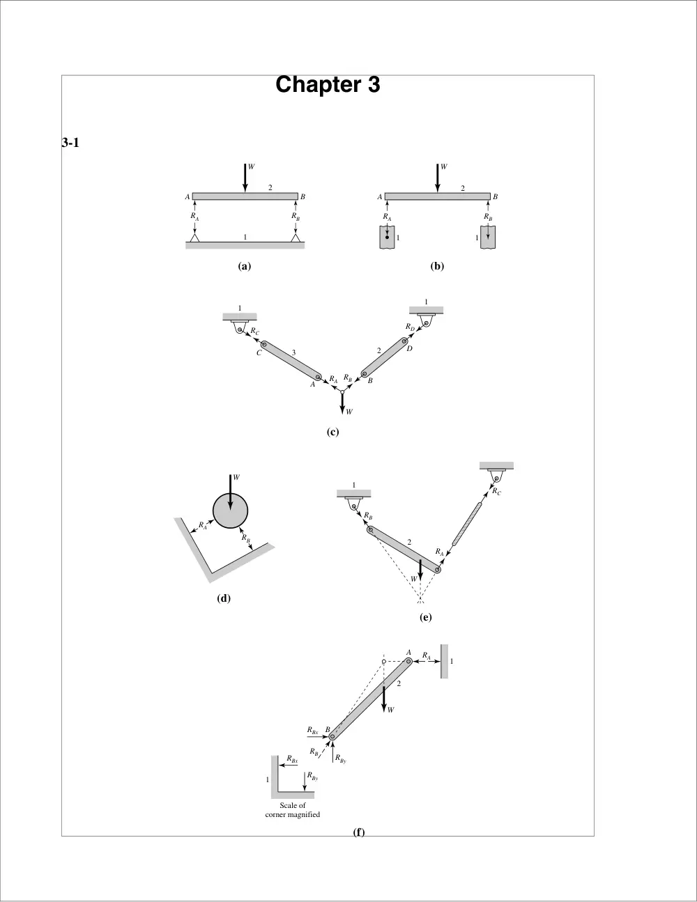
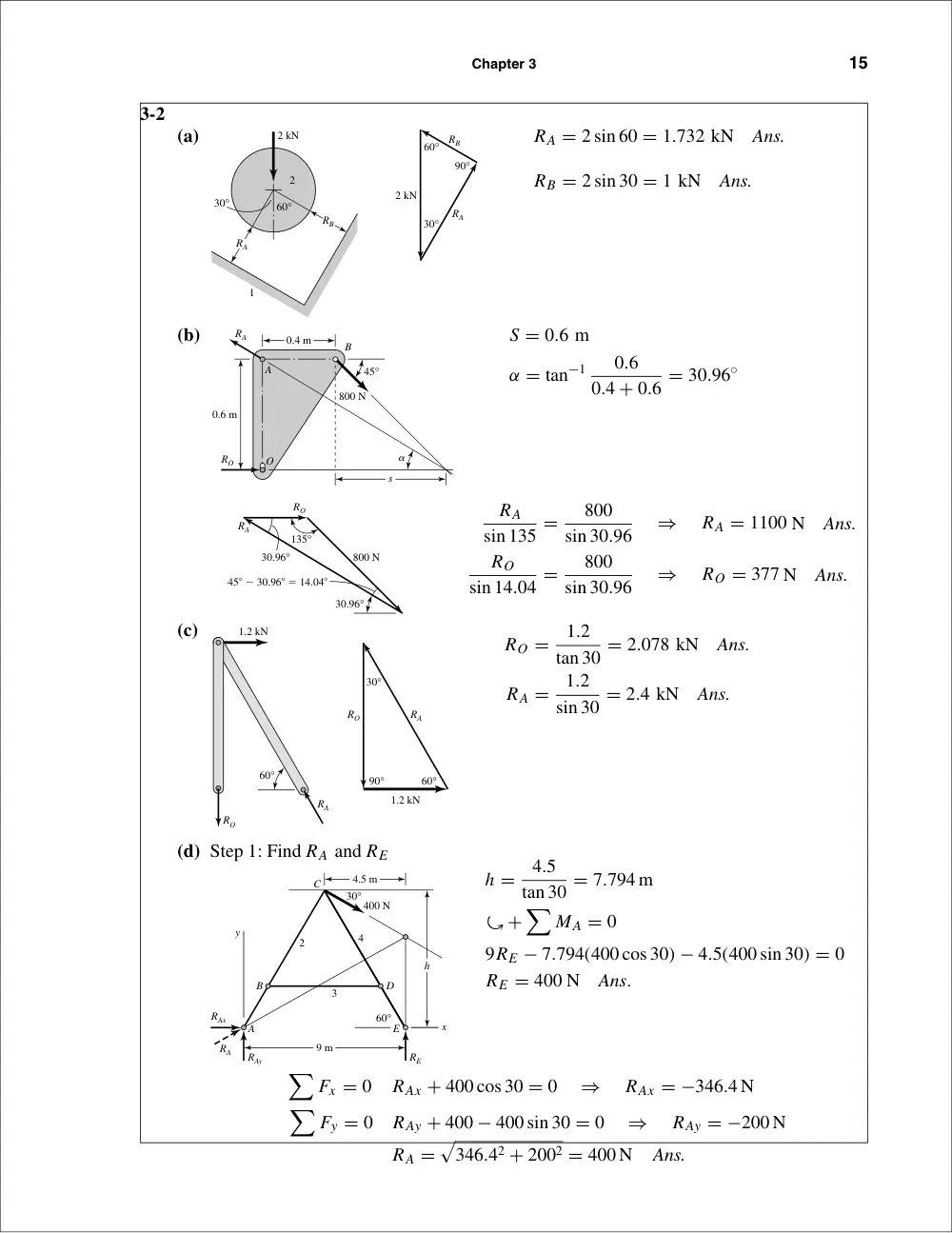
Chapter 3 3-1 1 RC RA RB RD C A B W D 1 2 3 RB RA W RB RC RA 2 1 W RA RBx RBx RBy RBy RB 2 1 1 Scale of corner magnified W A B (e) (f) (d) W A RA RB B 1 2 W A RA RB B 1 1 2 (a) (b) (c) Chapter 3 15 3-2 (a) RA = 2 sin 60 = 1.732 kN Ans. RB = 2 sin 30 = 1 kN Ans. (b) S = 0.6 m α = tan−1 0.6 0.4 + 0.6 = 30.96◦ RA sin 135 = 800 sin 30.96 ⇒ RA = 1100 N Ans. RO sin 14.04 = 800 sin 30.96 ⇒ RO = 377 N Ans. (c) RO = 1.2 tan 30 = 2.078 kN Ans. RA = 1.2 sin 30 = 2.4 kN Ans. (d) Step 1: Find RA and RE h = 4.5 tan 30 = 7.794 m �+ � MA = 0 9RE − 7.794(400 cos 30) − 4.5(400 sin 30) = 0 RE = 400 N Ans. � Fx = 0 RAx + 400 cos 30 = 0 ⇒ RAx = −346.4 N � Fy = 0 RAy + 400 − 400 sin 30 = 0 ⇒ RAy = −200 N RA = � 346.42 + 2002 = 400 N Ans. D C h B y E x A 4.5 m 9 m 400 N 3 4 2 30° 60° RAy RA RAx RE 1.2 kN 60° RA RO 60° 90° 30° 1.2 kN RA RO 45� � 30.96� � 14.04� 135° 30.96° 30.96° 800 N RA RO O 0.4 m 45° 800 N � 0.6 m A s RA RO B 60° 90° 30° 2 kN RA RB 2 1 2 kN 60° 30° RA RB 16 Solutions Manual • Instructor’s Solution Manual to Accompany Mechanical Engineering Design Step 2: Find components of RC on link 4 and RD �+ � MC = 0 400(4.5) − (7.794 − 1.9)RD = 0 ⇒ RD = 305.4 N Ans. � Fx = 0 ⇒ (RCx)4 = 305.4 N � Fy = 0 ⇒ (RCy)4 = −400 N Step 3: Find components of RC on link 2 � Fx = 0 (RCx)2 + 305.4 − 346.4 = 0 ⇒ (RCx)2 = 41 N � Fy = 0 (RCy)2 = 200 N 3-3 (a) �+ � M0 = 0 −18(60) + 14R2 + 8(30) − 4(40) = 0 R2 = 71.43 lbf � Fy = 0: R1 − 40 + 30 + 71.43 − 60 = 0 R1 = −1.43 lbf M1 = −1.43(4) = −5.72 lbf · in M2 = −5.72 − 41.43(4) = −171.44 lbf · in M3 = −171.44 − 11.43(6) = −240 lbf · in M4 = −240 + 60(4) = 0 checks! 4" 4" 6" 4" �1.43 �41.43 �11.43 60 40 lbf 60 lbf 30 lbf x x x O A B C D y R1 R2 M1 M2 M3 M4 O V (lbf) M (lbf•in) O C C D B A B D E 305.4 N 346.4 N 305.4 N 41 N 400 N 200 N 400 N 200 N 400 N Pin C 30° 305.4 N 400 N 400 N 200 N 41 N 305.4 N 200 N 346.4 N 305.4 N (RCx)2 (RCy)2 C B A 2 400 N 4 RD (RCx)4 (RCy)4 D C E Ans. 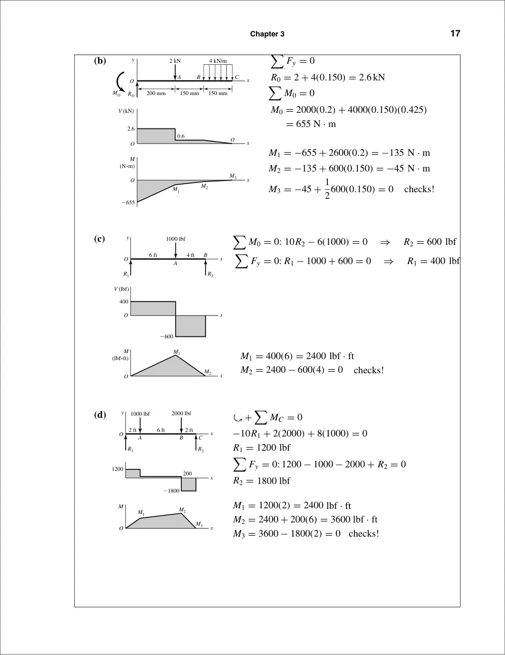Chapter 3 17 (b) � Fy = 0 R0 = 2 + 4(0.150) = 2.6kN � M0 = 0 M0 = 2000(0.2) + 4000(0.150)(0.425) = 655 N · m M1 = −655 + 2600(0.2) = −135 N · m M2 = −135 + 600(0.150) = −45 N · m M3 = −45 + 1 2600(0.150) = 0 checks! (c) � M0 = 0: 10R2 − 6(1000) = 0 ⇒ R2 = 600 lbf � Fy = 0: R1 − 1000 + 600 = 0 ⇒ R1 = 400 lbf M1 = 400(6) = 2400 lbf · ft M2 = 2400 − 600(4) = 0 checks! (d) �+ � MC = 0 −10R1 + 2(2000) + 8(1000) = 0 R1 = 1200 lbf � Fy = 0: 1200 − 1000 − 2000 + R2 = 0 R2 = 1800 lbf M1 = 1200(2) = 2400 lbf · ft M2 = 2400 + 200(6) = 3600 lbf · ft M3 = 3600 − 1800(2) = 0 checks! 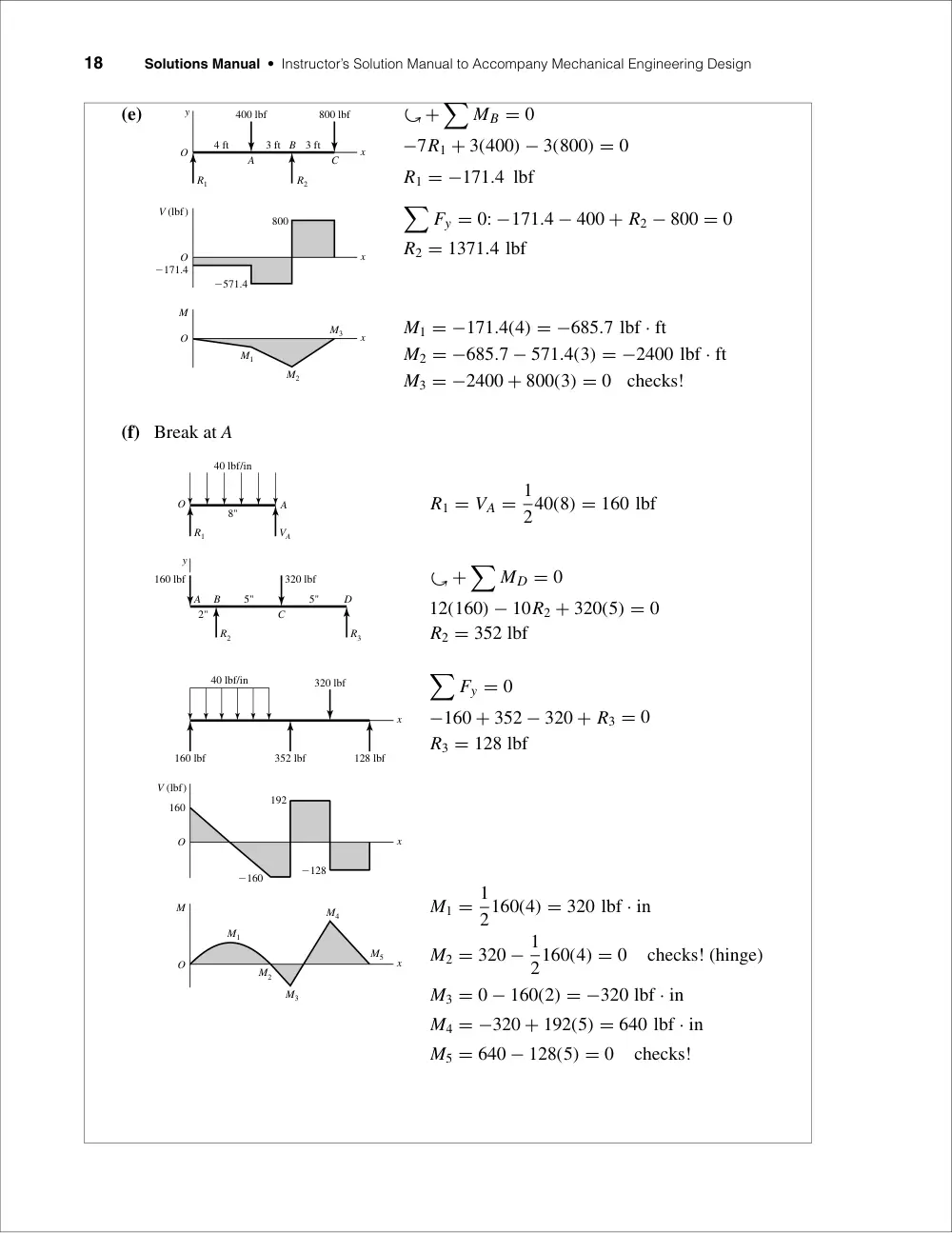2000 lbf 1000 lbf R1 O O M1 M2 M3 R2 6 ft 2 ft 2 ft A B C y M 1200 �1800 200 x x x 6 ft 4 ft A O O O B �600 M1 M2 V (lbf) 1000 lbf y R1 R2 400 M (lbf•ft) x x x V (kN) 150 mm 200 mm 150 mm 2.6 �655 M (N•m) 0.6 M1 M2 M3 2 kN 4 kN/m y A O O O O B C RO MO x x x 18 Solutions Manual • Instructor’s Solution Manual to Accompany Mechanical Engineering Design (e) �+ � MB = 0 −7R1 + 3(400) − 3(800) = 0 R1 = −171.4 lbf � Fy = 0: −171.4 − 400 + R2 − 800 = 0 R2 = 1371.4 lbf M1 = −171.4(4) = −685.7 lbf · ft M2 = −685.7 − 571.4(3) = −2400 lbf · ft M3 = −2400 + 800(3) = 0 checks! (f) Break at A R1 = VA = 1 240(8) = 160 lbf � + � MD = 0 12(160) − 10R2 + 320(5) = 0 R2 = 352 lbf � Fy = 0 −160 + 352 − 320 + R3 = 0 R3 = 128 lbf M1 = 1 2160(4) = 320 lbf · in M2 = 320 − 1 2160(4) = 0 checks! (hinge) M3 = 0 − 160(2) = −320 lbf · in M4 = −320 + 192(5) = 640 lbf · in M5 = 640 − 128(5) = 0 checks! 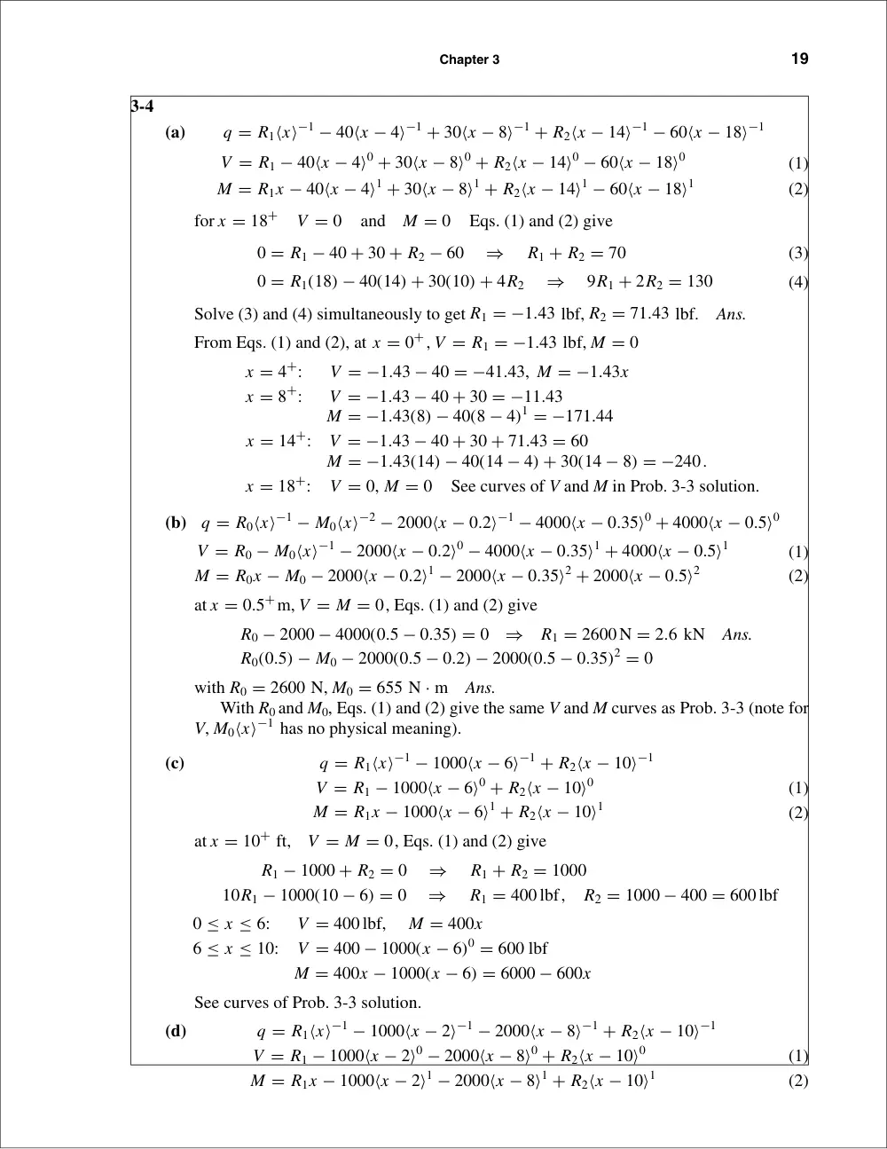40 lbf/in V (lbf) O O 160 �160 �128 192 M 320 lbf 160 lbf 352 lbf 128 lbf M1 M2 M3 M4 M5 x x x 8" 5" 2" 5" 40 lbf/in 160 lbf O A y B D C A 320 lbf R2 R3 R1 VA A O O O C M V (lbf) 800 �171.4 �571.4 3 ft 3 ft 4 ft 800 lbf 400 lbf B y M1 M2 M3 R1 R2 x x x Chapter 3 19 3-4 (a) q = R1⟨x⟩−1 − 40⟨x − 4⟩−1 + 30⟨x − 8⟩−1 + R2⟨x − 14⟩−1 − 60⟨x − 18⟩−1 V = R1 − 40⟨x − 4⟩0 + 30⟨x − 8⟩0 + R2⟨x − 14⟩0 − 60⟨x − 18⟩0 (1) M = R1x − 40⟨x − 4⟩1 + 30⟨x − 8⟩1 + R2⟨x − 14⟩1 − 60⟨x − 18⟩1 (2) for x = 18+ V = 0 and M = 0 Eqs. (1) and (2) give 0 = R1 − 40 + 30 + R2 − 60 ⇒ R1 + R2 = 70 (3) 0 = R1(18) − 40(14) + 30(10) + 4R2 ⇒ 9R1 + 2R2 = 130 (4) Solve (3) and (4) simultaneously to get R1 = −1.43 lbf, R2 = 71.43 lbf. Ans. From Eqs. (1) and (2), at x = 0+, V = R1 = −1.43 lbf, M = 0 x = 4+: V = −1.43 − 40 = −41.43, M = −1.43x x = 8+: V = −1.43 − 40 + 30 = −11.43 M = −1.43(8) − 40(8 − 4)1 = −171.44 x = 14+: V = −1.43 − 40 + 30 + 71.43 = 60 M = −1.43(14) − 40(14 − 4) + 30(14 − 8) = −240. x = 18+: V = 0, M = 0 See curves of V and M in Prob. 3-3 solution. (b) q = R0⟨x⟩−1 − M0⟨x⟩−2 − 2000⟨x − 0.2⟩−1 − 4000⟨x − 0.35⟩0 + 4000⟨x − 0.5⟩0 V = R0 − M0⟨x⟩−1 − 2000⟨x − 0.2⟩0 − 4000⟨x − 0.35⟩1 + 4000⟨x − 0.5⟩1 (1) M = R0x − M0 − 2000⟨x − 0.2⟩1 − 2000⟨x − 0.35⟩2 + 2000⟨x − 0.5⟩2 (2) at x = 0.5+m, V = M = 0, Eqs. (1) and (2) give R0 − 2000 − 4000(0.5 − 0.35) = 0 ⇒ R1 = 2600 N = 2.6 kN Ans. R0(0.5) − M0 − 2000(0.5 − 0.2) − 2000(0.5 − 0.35)2 = 0 with R0 = 2600 N, M0 = 655 N · m Ans. With R0 and M0, Eqs. (1) and (2) give the same V and M curves as Prob. 3-3 (note for V, M0⟨x⟩−1 has no physical meaning). (c) q = R1⟨x⟩−1 − 1000⟨x − 6⟩−1 + R2⟨x − 10⟩−1 V = R1 − 1000⟨x − 6⟩0 + R2⟨x − 10⟩0 (1) M = R1x − 1000⟨x − 6⟩1 + R2⟨x − 10⟩1 (2) at x = 10+ ft, V = M = 0, Eqs. (1) and (2) give R1 − 1000 + R2 = 0 ⇒ R1 + R2 = 1000 10R1 − 1000(10 − 6) = 0 ⇒ R1 = 400 lbf, R2 = 1000 − 400 = 600 lbf 0 ≤ x ≤ 6: V = 400 lbf, M = 400x 6 ≤ x ≤ 10: V = 400 − 1000(x − 6)0 = 600 lbf M = 400x − 1000(x − 6) = 6000 − 600x See curves of Prob. 3-3 solution. 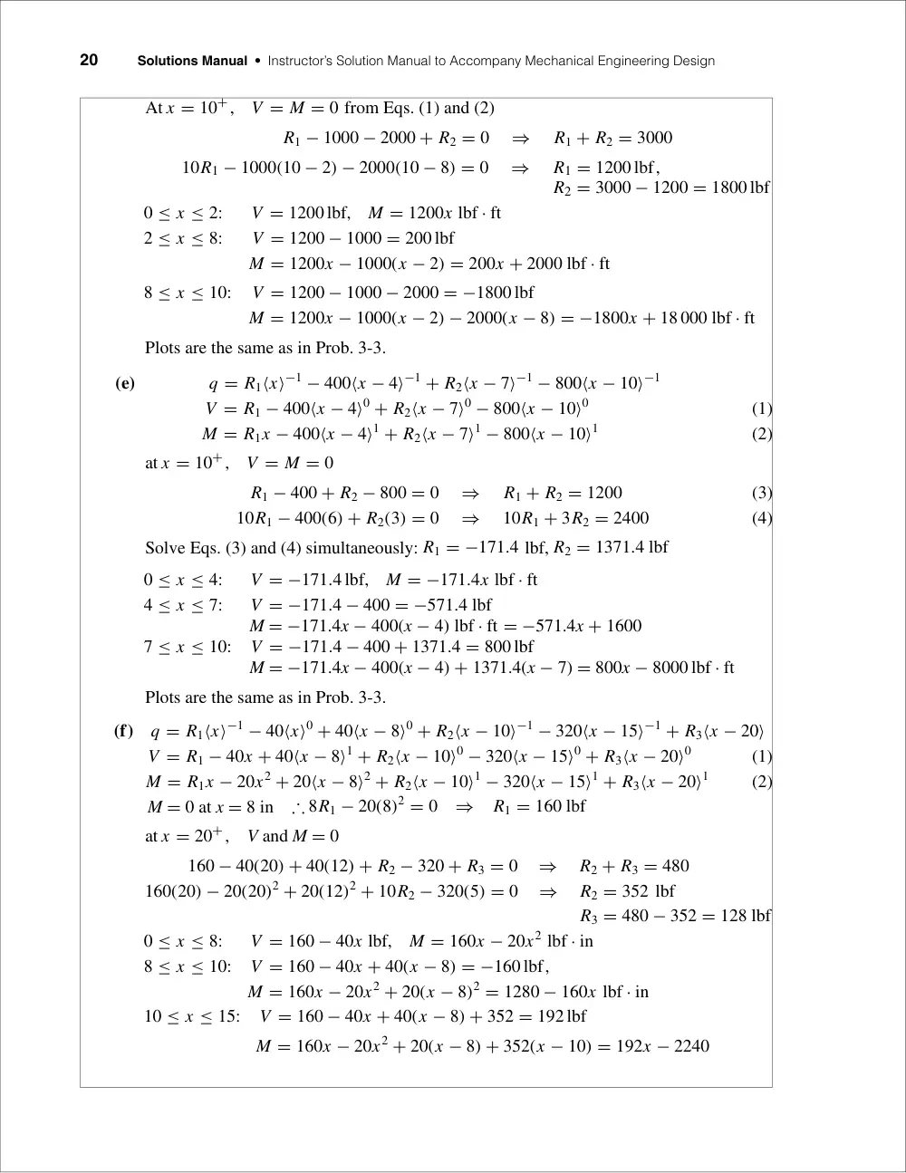(d) q = R1⟨x⟩−1 − 1000⟨x − 2⟩−1 − 2000⟨x − 8⟩−1 + R2⟨x − 10⟩−1 V = R1 − 1000⟨x − 2⟩0 − 2000⟨x − 8⟩0 + R2⟨x − 10⟩0 (1) M = R1x − 1000⟨x − 2⟩1 − 2000⟨x − 8⟩1 + R2⟨x − 10⟩1 (2) 20 Solutions Manual • Instructor’s Solution Manual to Accompany Mechanical Engineering Design At x = 10+, V = M = 0 from Eqs. (1) and (2) R1 − 1000 − 2000 + R2 = 0 ⇒ R1 + R2 = 3000 10R1 − 1000(10 − 2) − 2000(10 − 8) = 0 ⇒ R1 = 1200 lbf, R2 = 3000 − 1200 = 1800 lbf 0 ≤ x ≤ 2: V = 1200 lbf, M = 1200x lbf · ft 2 ≤ x ≤ 8: V = 1200 − 1000 = 200 lbf M = 1200x − 1000(x − 2) = 200x + 2000 lbf · ft 8 ≤ x ≤ 10: V = 1200 − 1000 − 2000 = −1800 lbf M = 1200x − 1000(x − 2) − 2000(x − 8) = −1800x + 18 000 lbf · ft Plots are the same as in Prob. 3-3. (e) q = R1⟨x⟩−1 − 400⟨x − 4⟩−1 + R2⟨x − 7⟩−1 − 800⟨x − 10⟩−1 V = R1 − 400⟨x − 4⟩0 + R2⟨x − 7⟩0 − 800⟨x − 10⟩0 (1) M = R1x − 400⟨x − 4⟩1 + R2⟨x − 7⟩1 − 800⟨x − 10⟩1 (2) at x = 10+, V = M = 0 R1 − 400 + R2 − 800 = 0 ⇒ R1 + R2 = 1200 (3) 10R1 − 400(6) + R2(3) = 0 ⇒ 10R1 + 3R2 = 2400 (4) Solve Eqs. (3) and (4) simultaneously: R1 = −171.4 lbf, R2 = 1371.4 lbf 0 ≤ x ≤ 4: V = −171.4 lbf, M = −171.4x lbf · ft 4 ≤ x ≤ 7: V = −171.4 − 400 = −571.4 lbf M = −171.4x − 400(x − 4) lbf · ft = −571.4x + 1600 7 ≤ x ≤ 10: V = −171.4 − 400 + 1371.4 = 800 lbf M = −171.4x − 400(x − 4) + 1371.4(x − 7) = 800x − 8000 lbf · ft Plots are the same as in Prob. 3-3. (f) q = R1⟨x⟩−1 − 40⟨x⟩0 + 40⟨x − 8⟩0 + R2⟨x − 10⟩−1 − 320⟨x − 15⟩−1 + R3⟨x − 20⟩ V = R1 − 40x + 40⟨x − 8⟩1 + R2⟨x − 10⟩0 − 320⟨x − 15⟩0 + R3⟨x − 20⟩0 (1) M = R1x − 20x2 + 20⟨x − 8⟩2 + R2⟨x − 10⟩1 − 320⟨x − 15⟩1 + R3⟨x − 20⟩1 (2) M = 0 at x = 8 in ∴ 8R1 − 20(8)2 = 0 ⇒ R1 = 160 lbf at x = 20+, V and M = 0 160 − 40(20) + 40(12) + R2 − 320 + R3 = 0 ⇒ R2 + R3 = 480 160(20) − 20(20)2 + 20(12)2 + 10R2 − 320(5) = 0 ⇒ R2 = 352 lbf R3 = 480 − 352 = 128 lbf 0 ≤ x ≤ 8: V = 160 − 40x lbf, M = 160x − 20x2 lbf · in 8 ≤ x ≤ 10: V = 160 − 40x + 40(x − 8) = −160 lbf, M = 160x − 20x2 + 20(x − 8)2 = 1280 − 160x lbf · in 10 ≤ x ≤ 15: V = 160 − 40x + 40(x − 8) + 352 = 192 lbf M = 160x − 20x2 + 20(x − 8) + 352(x − 10) = 192x − 2240 Chapter 3 21 15 ≤ x ≤ 20: V = 160 − 40x + 40(x − 8) + 352 − 320 = −128 lbf M = 160x − 20x2 − 20(x − 8) + 352(x − 10) − 320(x − 15) = −128x + 2560 Plots of V and M are the same as in Prob. 3-3. 3-5 Solution depends upon the beam selected. 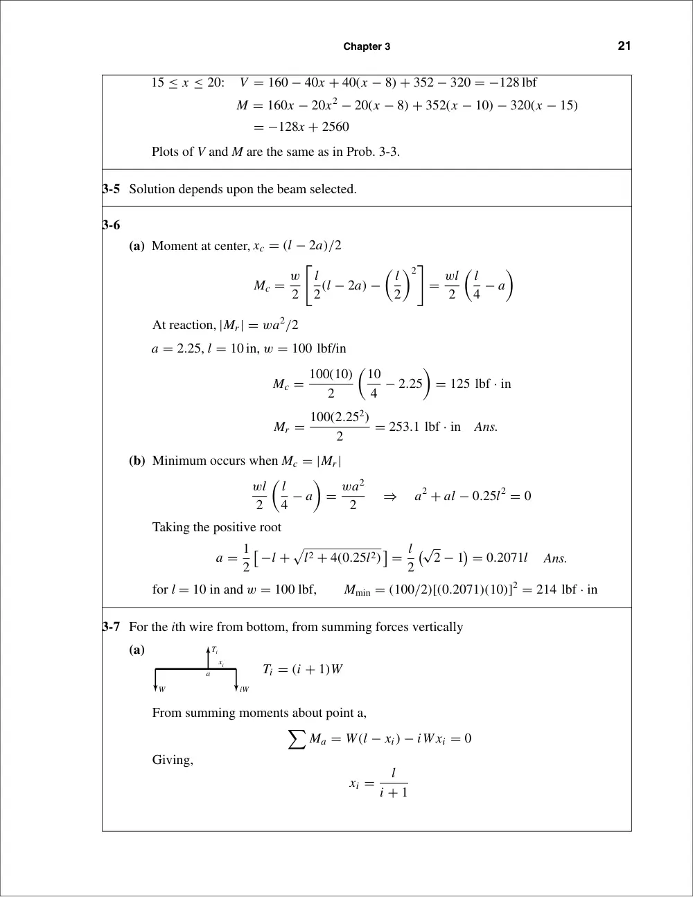3-6 (a) Moment at center, xc = (l − 2a)/2 Mc = w 2 � l 2(l − 2a) − � l 2 �2� = wl 2 � l 4 − a � At reaction, |Mr| = wa2/2 a = 2.25, l = 10 in, w = 100 lbf/in Mc = 100(10) 2 �10 4 − 2.25 � = 125 lbf · in Mr = 100(2.252) 2 = 253.1 lbf · in Ans. (b) Minimum occurs when Mc = |Mr| wl 2 � l 4 − a � = wa2 2 ⇒ a2 + al − 0.25l2 = 0 Taking the positive root a = 1 2 � −l + � l2 + 4(0.25l2) � = l 2 �√ 2 − 1 � = 0.2071l Ans. 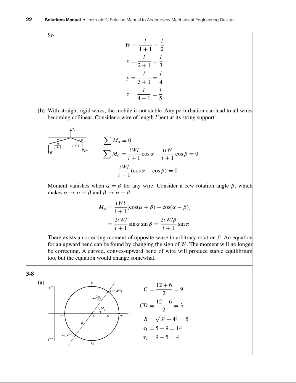for l = 10 in and w = 100 lbf, Mmin = (100/2)[(0.2071)(10)]2 = 214 lbf · in 3-7 For the ith wire from bottom, from summing forces vertically (a) Ti = (i + 1)W From summing moments about point a, � Ma = W(l − xi) − iW xi = 0 Giving, xi = l i + 1 W iW Ti xi a 22 Solutions Manual • Instructor’s Solution Manual to Accompany Mechanical Engineering Design So W = l 1 + 1 = l 2 x = l 2 + 1 = l 3 y = l 3 + 1 = l 4 z = l 4 + 1 = l 5 (b) With straight rigid wires, the mobile is not stable. Any perturbation can lead to all wires becoming collinear. Consider a wire of length l bent at its string support: � Ma = 0 � Ma = iWl i + 1 cos α − ilW i + 1 cos β = 0 iWl i + 1(cos α − cos β) = 0 Moment vanishes when α = β for any wire. Consider a ccw rotation angle β, which makes α → α + β and β → α − β Ma = iWl i + 1[cos(α + β) − cos(α − β)] = 2iWl i + 1 sin α sin β .= 2iWlβ i + 1 sin α There exists a correcting moment of opposite sense to arbitrary rotation β. An equation for an upward bend can be found by changing the sign of W. The moment will no longer be correcting. A curved, convex-upward bend of wire will produce stable equilibrium too, but the equation would change somewhat. 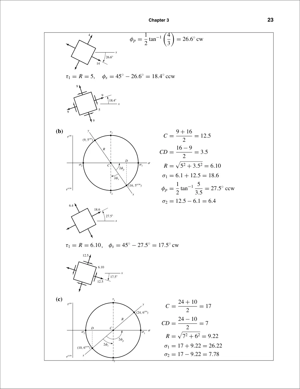3-8 (a) C = 12 + 6 2 = 9 CD = 12 − 6 2 = 3 R = � 32 + 42 = 5 σ1 = 5 + 9 = 14 σ2 = 9 − 5 = 4 2�s (12, 4cw) C R D �2 �1 �1 � �2 2�p (6, 4ccw) y x �cw �ccw W iW il i � 1 Ti � � l i � 1 Chapter 3 23 φp = 1 2 tan−1 �4 3 � = 26.6◦ cw τ1 = R = 5, φs = 45◦ − 26.6◦ = 18.4◦ ccw (b) C = 9 + 16 2 = 12.5 CD = 16 − 9 2 = 3.5 R = � 52 + 3.52 = 6.10 σ1 = 6.1 + 12.5 = 18.6 φp = 1 2 tan−1 5 3.5 = 27.5◦ ccw σ2 = 12.5 − 6.1 = 6.4 τ1 = R = 6.10, φs = 45◦ − 27.5◦ = 17.5◦ cw (c) C = 24 + 10 2 = 17 CD = 24 − 10 2 = 7 R = � 72 + 62 = 9.22 σ1 = 17 + 9.22 = 26.22 σ2 = 17 − 9.22 = 7.78 2�s (24, 6cw) C R D �2 �1 �1 �2 2�p (10, 6ccw) y x � �cw �ccw x 12.5 12.5 6.10 17.5� x 6.4 18.6 27.5� 2�s (16, 5ccw) C R D �2 �1 �1 �2 2�p (9, 5cw) y x � �cw �ccw 9 5 9 9 9 18.4� x x 4 14 26.6� 24 Solutions Manual • Instructor’s Solution Manual to Accompany Mechanical Engineering Design φp = 1 2 � 90 + tan−1 7 6 � = 69.7◦ ccw τ1 = R = 9.22, φs = 69.7◦ − 45◦ = 24.7◦ ccw (d) C = 9 + 19 2 = 14 CD = 19 − 9 2 = 5 R = � 52 + 82 = 9.434 σ1 = 14 + 9.43 = 23.43 σ2 = 14 − 9.43 = 4.57 φp = 1 2 � 90 + tan−1 5 8 � = 61.0◦ cw τ1 = R = 9.434, φs = 61◦ − 45◦ = 16◦ cw x 14 14 9.434 16� x 23.43 4.57 61� 2�s (9, 8cw) C R D �2 �1 �1 �2 2�p (19, 8ccw) y x � �cw �ccw x 17 17 9.22 24.7� x 26.22 7.78 69.7� Chapter 3 25 3-9 (a) C = 12 − 4 2 = 4 CD = 12 + 4 2 = 8 R = � 82 + 72 = 10.63 σ1 = 4 + 10.63 = 14.63 σ2 = 4 − 10.63 = −6.63 φp = 1 2 � 90 + tan−1 8 7 � = 69.4◦ ccw τ1 = R = 10.63, φs = 69.4◦ − 45◦ = 24.4◦ ccw (b) C = 6 − 5 2 = 0.5 CD = 6 + 5 2 = 5.5 R = � 5.52 + 82 = 9.71 σ1 = 0.5 + 9.71 = 10.21 σ2 = 0.5 − 9.71 = −9.21 φp = 1 2 tan−1 8 5.5 = 27.75◦ ccw x 10.21 9.21 27.75� 2�s (�5, 8cw) C R D �2 �1 �1 � �2 2�p (6, 8ccw) y x �cw �ccw x 4 4 10.63 24.4� x 14.63 6.63 69.4� 2�s (12, 7cw) C R D �2 �1 �1 � �2 2�p (�4, 7ccw) y x �cw �ccw 26 Solutions Manual • Instructor’s Solution Manual to Accompany Mechanical Engineering Design τ1 = R = 9.71, φs = 45◦ − 27.75◦ = 17.25◦ cw (c) C = −8 + 7 2 = −0.5 CD = 8 + 7 2 = 7.5 R = � 7.52 + 62 = 9.60 σ1 = 9.60 − 0.5 = 9.10 σ2 = −0.5 − 9.6 = −10.1 φp = 1 2 � 90 + tan−1 7.5 6 � = 70.67◦ cw τ1 = R = 9.60, φs = 70.67◦ − 45◦ = 25.67◦ cw (d) C = 9 − 6 2 = 1.5 CD = 9 + 6 2 = 7.5 R = � 7.52 + 32 = 8.078 σ1 = 1.5 + 8.078 = 9.58 σ2 = 1.5 − 8.078 = −6.58 2�s (9, 3cw) C R D �2 �1 �1 �2 2�p (�6, 3ccw) y x � �cw �ccw x 0.5 0.5 9.60 25.67� x 10.1 9.1 70.67� 2�s (�8, 6cw) C R D �2 �1 �1 �2 2�p (7, 6ccw) x y � �cw �ccw x 0.5 0.5 9.71 17.25� Chapter 3 27 φp = 1 2 tan−1 3 7.5 = 10.9◦ cw τ1 = R = 8.078, φs = 45◦ − 10.9◦ = 34.1◦ ccw 3-10 (a) C = 20 − 10 2 = 5 CD = 20 + 10 2 = 15 R = � 152 + 82 = 17 σ1 = 5 + 17 = 22 σ2 = 5 − 17 = −12 φp = 1 2 tan−1 8 15 = 14.04◦ cw τ1 = R = 17, φs = 45◦ − 14.04◦ = 30.96◦ ccw 5 17 5 30.96� x 12 22 14.04� x 2�s (20, 8cw) C R D �2 �1 �1 �2 2�p (�10, 8ccw) y x � �cw �ccw x 1.5 8.08 1.5 34.1� x 6.58 9.58 10.9� 28 Solutions Manual • Instructor’s Solution Manual to Accompany Mechanical Engineering Design (b) C = 30 − 10 2 = 10 CD = 30 + 10 2 = 20 R = � 202 + 102 = 22.36 σ1 = 10 + 22.36 = 32.36 σ2 = 10 − 22.36 = −12.36 φp = 1 2 tan−1 10 20 = 13.28◦ ccw τ1 = R = 22.36, φs = 45◦ − 13.28◦ = 31.72◦ cw (c) C = −10 + 18 2 = 4 CD = 10 + 18 2 = 14 R = � 142 + 92 = 16.64 σ1 = 4 + 16.64 = 20.64 σ2 = 4 − 16.64 = −12.64 φp = 1 2 � 90 + tan−1 14 9 � = 73.63◦ cw τ1 = R = 16.64, φs = 73.63◦ − 45◦ = 28.63◦ cw 4 x 16.64 4 28.63� 12.64 20.64 73.63� x 2�s (�10, 9cw) C R D �2 �1 �1 �2 2�p (18, 9ccw) y x � �cw �ccw 10 10 22.36 31.72� x 12.36 32.36 x 13.28� 2�s (�10, 10cw) C R D �2 �1 �1 � �2 2�p (30, 10ccw) y x �cw �ccw Chapter 3 29 (d) C = −12 + 22 2 = 5 CD = 12 + 22 2 = 17 R = � 172 + 122 = 20.81 σ1 = 5 + 20.81 = 25.81 σ2 = 5 − 20.81 = −15.81 φp = 1 2 � 90 + tan−1 17 12 � = 72.39◦ cw τ1 = R = 20.81, φs = 72.39◦ − 45◦ = 27.39◦ cw 3-11 (a) (b) C = 0 + 10 2 = 5 CD = 10 − 0 2 = 5 R = � 52 + 42 = 6.40 σ1 = 5 + 6.40 = 11.40 σ2 = 0, σ3 = 5 − 6.40 = −1.40 τ1/3 = R = 6.40, τ1/2 = 11.40 2 = 5.70, τ2/3 = 1.40 2 = 0.70 �1 �2 � �3 D x y � C R (0, 4cw) (10, 4ccw) �2/3 �1/2 �1/3 �x � �1 � �3 � �y � �2 � 0 �4 10 y x �2/3 � 2 �1/2 � 5 �1/3 � 14 � 7 2 5 20.81 5 27.39� x 15.81 25.81 72.39� x 2�s (�12, 12cw) C R D �2 �1 �1 �2 2�p (22, 12ccw) y x � �cw �ccw 30 Solutions Manual • Instructor’s Solution Manual to Accompany Mechanical Engineering Design (c) C = −2 − 8 2 = −5 CD = 8 − 2 2 = 3 R = � 32 + 42 = 5 σ1 = −5 + 5 = 0, σ2 = 0 σ3 = −5 − 5 = −10 τ1/3 = 10 2 = 5, τ1/2 = 0, τ2/3 = 5 (d) C = 10 − 30 2 = −10 CD = 10 + 30 2 = 20 R = � 202 + 102 = 22.36 σ1 = −10 + 22.36 = 12.36 σ2 = 0 σ3 = −10 − 22.36 = −32.36 τ1/3 = 22.36, τ1/2 = 12.36 2 = 6.18, τ2/3 = 32.36 2 = 16.18 3-12 (a) C = −80 − 30 2 = −55 CD = 80 − 30 2 = 25 R = � 252 + 202 = 32.02 σ1 = 0 σ2 = −55 + 32.02 = −22.98 = −23.0 σ3 = −55 − 32.0 = −87.0 τ1/2 = 23 2 = 11.5, τ2/3 = 32.0, τ1/3 = 87 2 = 43.5 �1 (�80, 20cw) (�30, 20ccw) C D R �2/3 �1/2 �1/3 �2 �3 x y � � �1 (�30, 10cw) (10, 10ccw) C D R �2/3 �1/2 � �1/3 �2 �3 � y x �1�2 � � �3 (�2, 4cw) Point is a circle 2 circles C D y x (�8, 4ccw) Chapter 3 31 (b) C = 30 − 60 2 = −15 CD = 60 + 30 2 = 45 R = � 452 + 302 = 54.1 σ1 = −15 + 54.1 = 39.1 σ2 = 0 σ3 = −15 − 54.1 = −69.1 τ1/3 = 39.1 + 69.1 2 = 54.1, τ1/2 = 39.1 2 = 19.6, τ2/3 = 69.1 2 = 34.6 (c) C = 40 + 0 2 = 20 CD = 40 − 0 2 = 20 R = � 202 + 202 = 28.3 σ1 = 20 + 28.3 = 48.3 σ2 = 20 − 28.3 = −8.3 σ3 = σz = −30 τ1/3 = 48.3 + 30 2 = 39.1, τ1/2 = 28.3, τ2/3 = 30 − 8.3 2 = 10.9 (d) C = 50 2 = 25 CD = 50 2 = 25 R = � 252 + 302 = 39.1 σ1 = 25 + 39.1 = 64.1 σ2 = 25 − 39.1 = −14.1 σ3 = σz = −20 τ1/3 = 64.1 + 20 2 = 42.1, τ1/2 = 39.1, τ2/3 = 20 − 14.1 2 = 2.95 �1 (50, 30cw) (0, 30ccw) C D �2/3 �1/2 �1/3 �2 �3 x y � � �1 (0, 20cw) (40, 20ccw) C D R �2/3 �1/2 �1/3 �2 �3 y x � � �1 � � (�60, 30ccw) (30, 30cw) C D R �2/3 �1/2 �1/3 �2 �3 x y 32 Solutions Manual • Instructor’s Solution Manual to Accompany Mechanical Engineering Design 3-13 σ = F A = 2000 (π/4)(0.52) = 10 190 psi = 10.19 kpsi Ans. δ = FL AE = σ L E = 10 190 72 30(106) = 0.024 46 in Ans. ϵ1 = δ L = 0.024 46 72 = 340(10−6) = 340µ Ans. From Table A-5, ν = 0.292 ϵ2 = −νϵ1 = −0.292(340) = −99.3µ Ans. �d = ϵ2d = −99.3(10−6)(0.5) = −49.6(10−6) in Ans. 3-14 From Table A-5, E = 71.7 GPa δ = σ L E = 135(106) 3 71.7(109) = 5.65(10−3) m = 5.65 mm Ans. 3-15 With σz = 0, solve the first two equations of Eq. (3-19) simultaneously. Place E on the left- hand side of both equations, and using Cramer’s rule, σx = ��� Eϵx −ν Eϵy 1 ��� ��� 1 −ν −ν 1 ��� = Eϵx + νEϵy 1 − ν2 = E(ϵx + νϵy) 1 − ν2 Likewise, σy = E(ϵy + νϵx) 1 − ν2 From Table A-5, E = 207 GPa and ν = 0.292. Thus, σx = E(ϵx + νϵy) 1 − ν2 = 207(109)[0.0021 + 0.292(−0.000 67)] 1 − 0.2922 (10−6) = 431 MPa Ans. σy = 207(109)[−0.000 67 + 0.292(0.0021)] 1 − 0.2922 (10−6) = −12.9 MPa Ans. 3-16 The engineer has assumed the stress to be uniform. That is, � Ft = −F cos θ + τ A = 0 ⇒ τ = F A cos θ When failure occurs in shear Ssu = F A cos θ � � t � F Chapter 3 33 The uniform stress assumption is common practice but is not exact. If interested in the details, see p. 570 of 6th edition. 3-17 From Eq. (3-15) σ 3 − (−2 + 6 − 4)σ 2 + [−2(6) + (−2)(−4) + 6(−4) − 32 − 22 − (−5)2]σ − [−2(6)(−4) + 2(3)(2)(−5) − (−2)(2)2 − 6(−5)2 − (−4)(3)2] = 0 σ 3 − 66σ + 118 = 0 Roots are: 7.012, 1.89, −8.903 kpsi Ans. τ1/2 = 7.012 − 1.89 2 = 2.56 kpsi τ2/3 = 8.903 + 1.89 2 = 5.40 kpsi τmax = τ1/3 = 8.903 + 7.012 2 = 7.96 kpsi Ans. Note: For Probs. 3-17 to 3-19, one can also find the eigenvalues of the matrix [σ] = � σx τxy τzx τxy σy τyz τzx τyz σz � for the principal stresses 3-18 From Eq. (3-15) σ 3 − (10 + 0 + 10)σ 2 + � 10(0) + 10(10) + 0(10) − 202 − � −10 √ 2 �2 − 02� σ − � 10(0)(10) + 2(20) � −10 √ 2 � (0) − 10 � −10 √ 2 �2 − 0(0)2 − 10(20)2� = 0 σ 3 − 20σ 2 − 500σ + 6000 = 0 Roots are: 30, 10, −20 MPa Ans. τ1/2 = 30 − 10 2 = 10 MPa τ2/3 = 10 + 20 2 = 15 MPa τmax = τ1/3 = 30 + 20 2 = 25 MPa Ans. 30 10 �20 �2/3 �1/2 �1/3 � (MPa) � (MPa) 7.012 1.89 �8.903 �2/3 �1/2 �1/3 � (kpsi) � (kpsi) 34 Solutions Manual • Instructor’s Solution Manual to Accompany Mechanical Engineering Design 3-19 From Eq. (3-15) σ 3 − (1 + 4 + 4)σ 2 + [1(4) + 1(4) + 4(4) − 22 − (−4)2 − (−2)2]σ −[1(4)(4) + 2(2)(−4)(−2) − 1(−4)2 − 4(−2)2 − 4(2)2] = 0 σ 3 − 9σ 2 = 0 Roots are: 9, 0, 0 kpsi τ2/3 = 0, τ1/2 = τ1/3 = τmax = 9 2 = 4.5 kpsi Ans. 3-20 (a) R1 = c l F Mmax = R1a = ac l F σ = 6M bh2 = 6 bh2 ac l F ⇒ F = σbh2l 6ac Ans. (b) Fm F = (σm/σ)(bm/b) (hm/h)2 (lm/l) (am/a) (cm/c) = 1(s)(s)2(s) (s)(s) = s2 Ans. For equal stress, the model load varies by the square of the scale factor. 3-21 R1 = wl 2 , Mmax|x=l/2 = w 2 l 2 � l − l 2 � = wl2 8 σ = 6M bh2 = 6 bh2 wl2 8 = 3Wl 4bh2 ⇒ W = 4 3 σbh2 l Ans. Wm W = (σm/σ)(bm/b) (hm/h)2 lm/l = 1(s)(s)2 s = s2 Ans. wmlm wl = s2 ⇒ wm w = s2 s = s Ans. For equal stress, the model load w varies linearily with the scale factor. �2/3 �(kpsi) �(kpsi) �1/2 � �1/3 O 0 9 Chapter 3 35 3-22 (a) Can solve by iteration or derive equations for the general case. Find maximum moment under wheel W3 WT = � W at centroid of W’s RA = l − x3 − d3 l WT Under wheel 3 M3 = RAx3 − W1a13 − W2a23 = (l − x3 − d3) l WT x3 − W1a13 − W2a23 For maximum, dM3 dx3 = 0 = (l − d3 − 2x3) WT l ⇒ x3 = l − d3 2 substitute into M, ⇒ M3 = (l − d3)2 4l WT − W1a13 − W2a23 This means the midpoint of d3 intersects the midpoint of the beam For wheel i xi = l − di 2 , Mi = (l − di)2 4l WT − i−1 � j=1 Wjaji Note for wheel 1: �Wjaji = 0 WT = 104.4, W1 = W2 = W3 = W4 = 104.4 4 = 26.1 kip Wheel 1: d1 = 476 2 = 238 in, M1 = (1200 − 238)2 4(1200) (104.4) = 20 128 kip · in Wheel 2: d2 = 238 − 84 = 154 in M2 = (1200 − 154)2 4(1200) (104.4) − 26.1(84) = 21 605 kip · in = Mmax Check if all of the wheels are on the rail (b) xmax = 600 − 77 = 523 in (c) See above sketch. (d) inner axles 600" 600" 84" 77" 84" 315" xmax RA W1 A B W3 . . . . . . W2 WT d3 Wn RB a23 a13 x3 l 36 Solutions Manual • Instructor’s Solution Manual to Accompany Mechanical Engineering Design 3-23 (a) Aa = Ab = 0.25(1.5) = 0.375 in2 A = 3(0.375) = 1.125 in2 ¯y = 2(0.375)(0.75) + 0.375(0.5) 1.125 = 0.667 in Ia = 0.25(1.5)3 12 = 0.0703 in4 Ib = 1.5(0.25)3 12 = 0.001 95 in4 I1 = 2[0.0703 + 0.375(0.083)2] + [0.001 95 + 0.375(0.167)2] = 0.158 in4 Ans. σA = 10 000(0.667) 0.158 = 42(10)3 psi Ans. σB = 10 000(0.667 − 0.375) 0.158 = 18.5(10)3 psi Ans. σC = 10 000(0.167 − 0.125) 0.158 = 2.7(10)3 psi Ans. σD = −10 000(0.833) 0.158 = −52.7(10)3 psi Ans. (b) Here we treat the hole as a negative area. Aa = 1.732 in2 Ab = 1.134 �0.982 2 � = 0.557 in2 D C B A y 1 1 a b A Ga Gb 0.327" 0.25" c1 � 1.155" c2 � 0.577" 2" 1.732" 0.577" 0.982" 0.577" 1.134" 1 2 1 " 1 4" 3 8" 1 4" 1 4" D C 1 1 Ga Gb c1 � 0.833" 0.167" 0.083" 0.5" 0.75" 1.5" y � c2 � 0.667" B a a b A Chapter 3 37 A = 1.732 − 0.557 = 1.175 in2 ¯y = 1.732(0.577) − 0.557(0.577) 1.175 = 0.577 in Ans. Ia = bh3 36 = 2(1.732)3 36 = 0.289 in4 Ib = 1.134(0.982)3 36 = 0.0298 in4 I1 = Ia − Ib = 0.289 − 0.0298 = 0.259 in4 Ans. because the centroids are coincident. σA = 10 000(0.577) 0.259 = 22.3(10)3 psi Ans. σB = 10 000(0.327) 0.259 = 12.6(10)3 psi Ans. σC = −10 000(0.982 − 0.327) 0.259 = −25.3(10)3 psi Ans. σD = −10 000(1.155) 0.259 = −44.6(10)3 psi Ans. (c) Use two negative areas. Aa = 1 in2, Ab = 9 in2, Ac = 16 in2, A = 16 − 9 − 1 = 6 in2; ¯ya = 0.25 in, ¯yb = 2.0 in, ¯yc = 2 in ¯y = 16(2) − 9(2) − 1(0.25) 6 = 2.292 in Ans. c1 = 4 − 2.292 = 1.708 in Ia = 2(0.5)3 12 = 0.020 83 in4 Ib = 3(3)3 12 = 6.75 in4 Ic = 4(4)3 12 = 21.333 in4 D C c a B b A Ga Gb Gc c1 � 1.708" c2 � 2.292" 2" 1.5" 0.25" 1 1 38 Solutions Manual • Instructor’s Solution Manual to Accompany Mechanical Engineering Design I1 = [21.333 + 16(0.292)2] − [6.75 + 9(0.292)2] − [0.020 83 + 1(2.292 − 0.25)2] = 10.99 in4 Ans. σA = 10 000(2.292) 10.99 = 2086 psi Ans. σB = 10 000(2.292 − 0.5) 10.99 = 1631 psi Ans. σC = −10 000(1.708 − 0.5) 10.99 = −1099 psi Ans. σD = −10 000(1.708) 10.99 = −1554 psi Ans. (d) Use a as a negative area. Aa = 6.928 in2, Ab = 16 in2, A = 9.072 in2; ¯ya = 1.155 in, ¯yb = 2 in ¯y = 2(16) − 1.155(6.928) 9.072 = 2.645 in Ans. c1 = 4 − 2.645 = 1.355 in Ia = bh3 36 = 4(3.464)3 36 = 4.618 in4 Ib = 4(4)3 12 = 21.33 in4 I1 = [21.33 + 16(0.645)2] − [4.618 + 6.928(1.490)2] = 7.99 in4 Ans. σA = 10 000(2.645) 7.99 = 3310 psi Ans. σB = −10 000(3.464 − 2.645) 7.99 = −1025 psi Ans. σC = −10 000(1.355) 7.99 = −1696 psi Ans. 3.464" 1 1 Ga B b a C A c1 � 1.355" c2 � 2.645" 1.490" 1.155" Chapter 3 39 (e) Aa = 6(1.25) = 7.5 in2 Ab = 3(1.5) = 4.5 in2 A = Ac + Ab = 12 in2 ¯y = 3.625(7.5) + 1.5(4.5) 12 = 2.828 in Ans. I = 1 12(6)(1.25)3 + 7.5(3.625 − 2.828)2 + 1 12(1.5)(3)3 + 4.5(2.828 − 1.5)2 = 17.05 in4 Ans. σA = 10 000(2.828) 17.05 = 1659 psi Ans. σB = −10 000(3 − 2.828) 17.05 = −101 psi Ans. σC = −10 000(1.422) 17.05 = −834 psi Ans. (f) Let a = total area A = 1.5(3) − 1(1.25) = 3.25 in2 I = Ia − 2Ib = 1 12(1.5)(3)3 − 1 12(1.25)(1)3 = 3.271 in4 Ans. σA = 10 000(1.5) 3.271 = 4586 psi, σD = −4586 psi Ans. σB = 10 000(0.5) 3.271 = 1529 psi, σC = −1529 psi 3-24 (a) The moment is maximum and constant between A and B M = −50(20) = −1000 lbf · in, I = 1 12(0.5)(2)3 = 0.3333 in4 ρ = ���� E I M ���� = 1.6(106)(0.3333) 1000 = 533.3 in (x, y) = (30, −533.3) in Ans. (b) The moment is maximum and constant between A and B M = 50(5) = 250 lbf · in, I = 0.3333 in4 ρ = 1.6(106)(0.3333) 250 = 2133 in Ans. (x, y) = (20, 2133) in Ans. C B A b a b D c � 1.5 c � 1.5 1.5 a b A B C c1 � 1.422" c2 � 2.828" 40 Solutions Manual • Instructor’s Solution Manual to Accompany Mechanical Engineering Design 3-25 (a) I = 1 12(0.75)(1.5)3 = 0.2109 in4 A = 0.75(1.5) = 1.125 in Mmax is at A. At the bottom of the section, σmax = Mc I = 4000(0.75) 0.2109 = 14 225 psi Ans. Due to V, τmax constant is between A and B at y = 0 τmax = 3 2 V A = 3 2 667 1.125 = 889 psi Ans. (b) I = 1 12(1)(2)3 = 0.6667 in4 Mmax is at A at the top of the beam σmax = 8000(1) 0.6667 = 12 000 psi Ans. |Vmax| = 1000 lbf from O to B at y = 0 τmax = 3 2 V A = 3 2 1000 (2)(1) = 750 psi Ans. (c) I = 1 12(0.75)(2)3 = 0.5 in4 M1 = −1 2600(5) = −1500 lbf · in = M3 M2 = −1500 + 1 2(900)(7.5) = 1875 lbf · in Mmax is at span center. At the bottom of the beam, σmax = 1875(1) 0.5 = 3750 psi Ans. At A and B at y = 0 τmax = 3 2 900 (0.75)(2) = 900 psi Ans. 120 lbf/in 1500 lbf 1500 lbf O C B A O O V (lbf) M (lbf•in) 5" 15" 5" 900 M1 M2 x M3 �900 �600 600 x x 1000 lbf 1000 lbf 1000 �1000 �8000 2000 lbf O B A O O 8" 8" V (lbf) M (lbf•in) x x x 1000 lbf 4000 333 lbf 667 lbf O B x A O 333 667 O 12" 6" V (lbf) M (lbf•in) x Chapter 3 41 (d) I = 1 12(1)(2)3 = 0.6667 in4 M1 = −600 2 (6) = −1800 lbf · in M2 = −1800 + 1 2750(7.5) = 1013 lbf · in At A, top of beam σmax = 1800(1) 0.6667 = 2700 psi Ans. At A, y = 0 τmax = 3 2 750 (2)(1) = 563 psi Ans. 3-26 Mmax = wl2 8 ⇒ σmax = wl2c 8I ⇒ w = 8σ I cl2 (a) l = 12(12) = 144 in, I = (1/12)(1.5)(9.5)3 = 107.2 in4 w = 8(1200)(107.2) 4.75(1442) = 10.4 lbf/in Ans. (b) l = 48 in, I = (π/64)(24 − 1.254) = 0.6656 in4 w = 8(12)(103)(0.6656) 1(48)2 = 27.7 lbf/in Ans. (c) l = 48 in, I .= (1/12)(2)(33) − (1/12)(1.625)(2.6253) = 2.051 in4 w = 8(12)(103)(2.051) 1.5(48)2 = 57.0 lbf/in Ans. (d) l = 72 in; Table A-6, I = 2(1.24) = 2.48 in4 cmax = 2.158" w = 8(12)(103)(2.48) 2.158(72)2 = 21.3 lbf/in Ans. (e) l = 72 in; Table A-7, I = 3.85 in4 w = 8(12)(103)(3.85) 2(722) = 35.6 lbf/in Ans. (f) l = 72 in, I = (1/12)(1)(43) = 5.333 in4 w = 8(12)(103)(5.333) (2)(72)2 = 49.4 lbf/in Ans. 2 0.842" 2.158" 100 lbf/in 1350 lbf 450 lbf O B A O O V (lbf) M (lbf•in) 6" 12" 7.5" 750 M1 M2 �450 �600 x x x 42 Solutions Manual • Instructor’s Solution Manual to Accompany Mechanical Engineering Design 3-27 (a) Model (c) I = π 64(0.54) = 3.068(10−3) in4 A = π 4 (0.52) = 0.1963 in2 σ = Mc I = 218.75(0.25) 3.068(10−3) = 17 825 psi = 17.8 kpsi Ans. τmax = 4 3 V A = 4 3 500 0.1963 = 3400 psi Ans. (b) Model (d) Mmax = 500(0.25) + 1 2(500)(0.375) = 218.75 lbf · in Vmax = 500 lbf Same M and V ∴ σ = 17.8 kpsi Ans. τmax = 3400 psi Ans. 3-28 q = −F⟨x⟩−1 + p1⟨x − l⟩0 − p1 + p2 a ⟨x − l⟩1 + terms for x > l + a V = −F + p1⟨x − l⟩1 − p1 + p2 2a ⟨x − l⟩2 + terms for x > l + a M = −Fx + p1 2 ⟨x − l⟩2 − p1 + p2 6a ⟨x − l⟩3 + terms for x > l + a At x = (l + a)+, V = M = 0, terms for x > l + a = 0 −F + p1a − p1 + p2 2a a2 = 0 ⇒ p1 − p2 = 2F a (1) l p2 p1 a b F 1.25" 500 lbf 500 lbf 0.25" 1333 lbf/in 500 �500 O V (lbf) O M Mmax 1.25 in 500 lbf 500 lbf 500 lbf 500 lbf 0.4375 500 �500 O V (lbf) O M (lbf•in) Mmax � 500(0.4375) � 218.75 lbf•in Chapter 3 43 −F(l + a) + p1a2 2 − p1 + p2 6a a3 = 0 ⇒ 2p1 − p2 = 6F(l + a) a2 (2) From (1) and (2) p1 = 2F a2 (3l + 2a), p2 = 2F a2 (3l + a) (3) From similar triangles b p2 = a p1 + p2 ⇒ b = ap2 p1 + p2 (4) Mmax occurs where V = 0 xmax = l + a − 2b Mmax = −F(l + a − 2b) + p1 2 (a − 2b)2 − p1 + p2 6a (a − 2b)3 = −Fl − F(a − 2b) + p1 2 (a − 2b)2 − p1 + p2 6a (a − 2b)3 Normally Mmax = −Fl The fractional increase in the magnitude is � = F(a − 2b) − ( p1/2)(a − 2b)2 − [( p1 + p2)/6a](a − 2b)3 Fl (5) For example, consider F = 1500 lbf, a = 1.2 in, l = 1.5 in (3) p1 = 2(1500) 1.22 [3(1.5) + 2(1.2)] = 14 375 lbf/in p2 = 2(1500) 1.22 [3(1.5) + 1.2] = 11 875 lbf/in (4) b = 1.2(11 875)/(14 375 + 11 875) = 0.5429 in Substituting into (5) yields � = 0.036 89 or 3.7% higher than −Fl a � 2b l F p2 p2 p1 p2 b b 3-29 R1 = 600(15) 2 + 20 153000 = 8500 lbf R2 = 600(15) 2 − 5 153000 = 3500 lbf a = 3500 600 = 5.833 ft (a) ¯y = 1(12) + 5(12) 24 = 3 in Iz = 1 3[2(53) + 6(33) − 4(13)] = 136 in4 At x = 5 ft, y = −3 in, σx = −−15000(12)(−3) 136 = −3970 psi y = 5 in, σx = −−15000(12)5 136 = 6620 psi At x = 14.17 ft, y = −3 in, σx = −20420(12)(−3) 136 = 5405 psi y = 5 in, σx = −20420(12)5 136 = −9010 psi Max tension = 6620 psi Ans. Max compression = −9010 psi Ans. (b) Vmax = 5500 lbf Qn.a. = ¯yA = 2.5(5)(2) = 25 in3 τmax = V Q Ib = 5500(25) 136(2) = 506 psi Ans. (c) τmax = |σmax| 2 = 9010 2 = 4510 psi Ans. z 5 in 44 Solutions Manual • Instructor’s Solution Manual to Accompany Mechanical Engineering Design 600 lbf/ft 3000 lbf O O V (lbf) M (lbf•ft) 5' 15' R1 R2 �3000 �3500 3500(5.833) � 20420 �15000 5500 x y x x a z y y V 3-30 R1 = c l F M = c l Fx 0 ≤ x ≤ a σ = 6M bh2 = 6(c/l)Fx bh2 ⇒ h = � 6cFx blσmax 0 ≤ x ≤ a Ans. 3-31 From Prob. 3-30, R1 = c l F = V, 0 ≤ x ≤ a τmax = 3 2 V bh = 3 2 (c/l)F bh ∴ h = 3 2 Fc lbτmax Ans. From Prob. 3-30 = � 6Fcx lbσmax sub in x = e and equate to h above 3 2 Fc lbτmax = � 6Fce lbσmax e = 3 8 Fcσmax lbτ 2max Ans. 3-32 R1 = b l F M = b l Fx σmax = 32M πd3 = 32 πd3 b l Fx d = �32 π bFx lσmax �1/3 0 ≤ x ≤ a Ans. 3-33 Square: Am = (b − t)2 Tsq = 2Amtτall = 2(b − t)2tτall Round: Am = π(b − t)2/4 Trd = 2π(b − t)2tτall/4 t b t b R1 F a b l R2 x y R1 R2 F a c l h(x) x e h Chapter 3 45 46 Solutions Manual • Instructor’s Solution Manual to Accompany Mechanical Engineering Design Ratio of torques Tsq Trd = 2(b − t)2tτall π(b − t)2tτall/2 = 4 π = 1.27 Twist per unit length square: θsq = 2Gθ1t tτall � L A � m = C ���� L A ���� m = C 4(b − t) (b − t)2 Round: θrd = C � L A � m = C π(b − t) π(b − t)2/4 = C 4(b − t) (b − t)2 Ratio equals 1, twists are the same. Note the weight ratio is Wsq Wrd = ρl(b − t)2 ρlπ(b − t)(t) = b − t πt thin-walled assumes b ≥ 20t = 19 π = 6.04 with b = 20t = 2.86 with b = 10t 3-34 l = 40 in, τall = 11 500 psi, G = 11.5(106) psi, t = 0.050 in rm = ri + t/2 = ri + 0.025 for ri > 0 = 0 for ri = 0 Am = (1 − 0.05)2 − 4 � r2 m − π 4 r2 m � = 0.952 − (4 − π)r2 m Lm = 4(1 − 0.05 − 2rm + 2πrm/4) = 4[0.95 − (2 − π/2)rm] Eq. (3-45): T = 2Amtτ = 2(0.05)(11 500)Am = 1150Am Eq. (3-46): θ(deg) = θ1 l 180 π = T Lml 4G A2mt 180 π = T Lm(40) 4(11.5)(106)A2m(0.05) 180 π = 9.9645(10−4) T Lm A2m Equations can then be put into a spreadsheet resulting in: ri rm Am Lm ri T(lbf · in) ri θ(deg) 0 0 0.902 5 3.8 0 1037.9 0 4.825 0.10 0.125 0.889 087 3.585398 0.10 1022.5 0.10 4.621 0.20 0.225 0.859 043 3.413717 0.20 987.9 0.20 4.553 0.30 0.325 0.811 831 3.242035 0.30 933.6 0.30 4.576 0.40 0.425 0.747 450 3.070354 0.40 859.6 0.40 4.707 0.45 0.475 0.708 822 2.984513 0.45 815.1 0.45 4.825 Chapter 3 47 Torque carrying capacity reduces with ri. However, this is based on an assumption of uni- form stresses which is not the case for small ri. Also note that weight also goes down with an increase in ri. 3-35 From Eq. (3-47) where θ1 is the same for each leg. T1 = 1 3Gθ1L1c3 1, T2 = 1 3Gθ1L2c3 2 T = T1 + T2 = 1 3Gθ1 � L1c3 1 + L2c3 2 � = 1 3Gθ1 � Lic3 i Ans. τ1 = Gθ1c1, τ2 = Gθ1c2 τmax = Gθ1cmax Ans. 3-36 (a) τmax = Gθ1cmax Gθ1 = τmax cmax = 12 000 1/8 = 9.6(104) psi/in T1/16 = 1 3Gθ1(Lc3)1/16 = 1 3(9.6)(104)(5/8)(1/16)3 = 4.88 lbf · in Ans. ri (in) � (deg) 4.50 4.55 4.65 4.60 4.70 4.75 4.80 4.85 0 0.3 0.2 0.1 0.4 0.5 ri (in) T (lbf•in) 0 400 200 600 800 1000 1200 0 0.3 0.2 0.1 0.4 0.5 48 Solutions Manual • Instructor’s Solution Manual to Accompany Mechanical Engineering Design T1/8 = 1 3(9.6)(104)(