STAT 230 Problems, Summer 2011

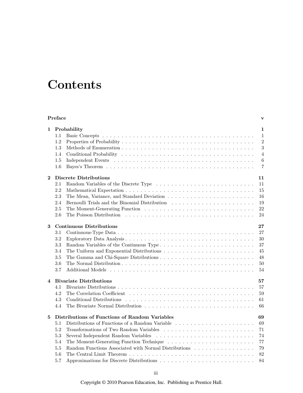
Contents Preface v 1 Probability 1 1.1 Basic Concepts . . . . . . . . . . . . . . . . . . . . . . . . . . . . . . . . . . . . . . . . 1 1.2 Properties of Probability . . . . . . . . . . . . . . . . . . . . . . . . . . . . . . . . . . . 2 1.3 Methods of Enumeration . . . . . . . . . . . . . . . . . . . . . . . . . . . . . . . . . . . 3 1.4 Conditional Probability . . . . . . . . . . . . . . . . . . . . . . . . . . . . . . . . . . . 4 1.5 Independent Events . . . . . . . . . . . . . . . . . . . . . . . . . . . . . . . . . . . . . 6 1.6 Bayes’s Theorem . . . . . . . . . . . . . . . . . . . . . . . . . . . . . . . . . . . . . . . 7 2 Discrete Distributions 11 2.1 Random Variables of the Discrete Type . . . . . . . . . . . . . . . . . . . . . . . . . . 11 2.2 Mathematical Expectation . . . . . . . . . . . . . . . . . . . . . . . . . . . . . . . . . . 15 2.3 The Mean, Variance, and Standard Deviation . . . . . . . . . . . . . . . . . . . . . . . 16 2.4 Bernoulli Trials and the Binomial Distribution . . . . . . . . . . . . . . . . . . . . . . 19 2.5 The Moment-Generating Function . . . . . . . . . . . . . . . . . . . . . . . . . . . . . 22 2.6 The Poisson Distribution . . . . . . . . . . . . . . . . . . . . . . . . . . . . . . . . . . 24 3 Continuous Distributions 27 3.1 Continuous-Type Data . . . . . . . . . . . . . . . . . . . . . . . . . . . . . . . . . . . . 27 3.2 Exploratory Data Analysis . . . . . . . . . . . . . . . . . . . . . . . . . . . . . . . . . . 30 3.3 Random Variables of the Continuous Type . . . . . . . . . . . . . . . . . . . . . . . . . 37 3.4 The Uniform and Exponential Distributions . . . . . . . . . . . . . . . . . . . . . . . . 45 3.5 The Gamma and Chi-Square Distributions . . . . . . . . . . . . . . . . . . . . . . . . . 48 3.6 The Normal Distribution . . . . . . . . . . . . . . . . . . . . . . . . . . . . . . . . . . . 50 3.7 Additional Models . . . . . . . . . . . . . . . . . . . . . . . . . . . . . . . . . . . . . . 54 4 Bivariate Distributions 57 4.1 Bivariate Distributions . . . . . . . . . . . . . . . . . . . . . . . . . . . . . . . . . . . . 57 4.2 The Correlation Coefficient . . . . . . . . . . . . . . . . . . . . . . . . . . . . . . . . . 59 4.3 Conditional Distributions . . . . . . . . . . . . . . . . . . . . . . . . . . . . . . . . . . 61 4.4 The Bivariate Normal Distribution . . . . . . . . . . . . . . . . . . . . . . . . . . . . . 66 5 Distributions of Functions of Random Variables 69 5.1 Distributions of Functions of a Random Variable . . . . . . . . . . . . . . . . . . . . . 69 5.2 Transformations of Two Random Variables . . . . . . . . . . . . . . . . . . . . . . . . 71 5.3 Several Independent Random Variables . . . . . . . . . . . . . . . . . . . . . . . . . . 74 5.4 The Moment-Generating Function Technique . . . . . . . . . . . . . . . . . . . . . . . 77 5.5 Random Functions Associated with Normal Distributions . . . . . . . . . . . . . . . . 79 5.6 The Central Limit Theorem . . . . . . . . . . . . . . . . . . . . . . . . . . . . . . . . . 82 5.7 Approximations for Discrete Distributions . . . . . . . . . . . . . . . . . . . . . . . . . 84 iii Copyright © 2010 Pearson Education, Inc. Publishing as Prentice Hall. 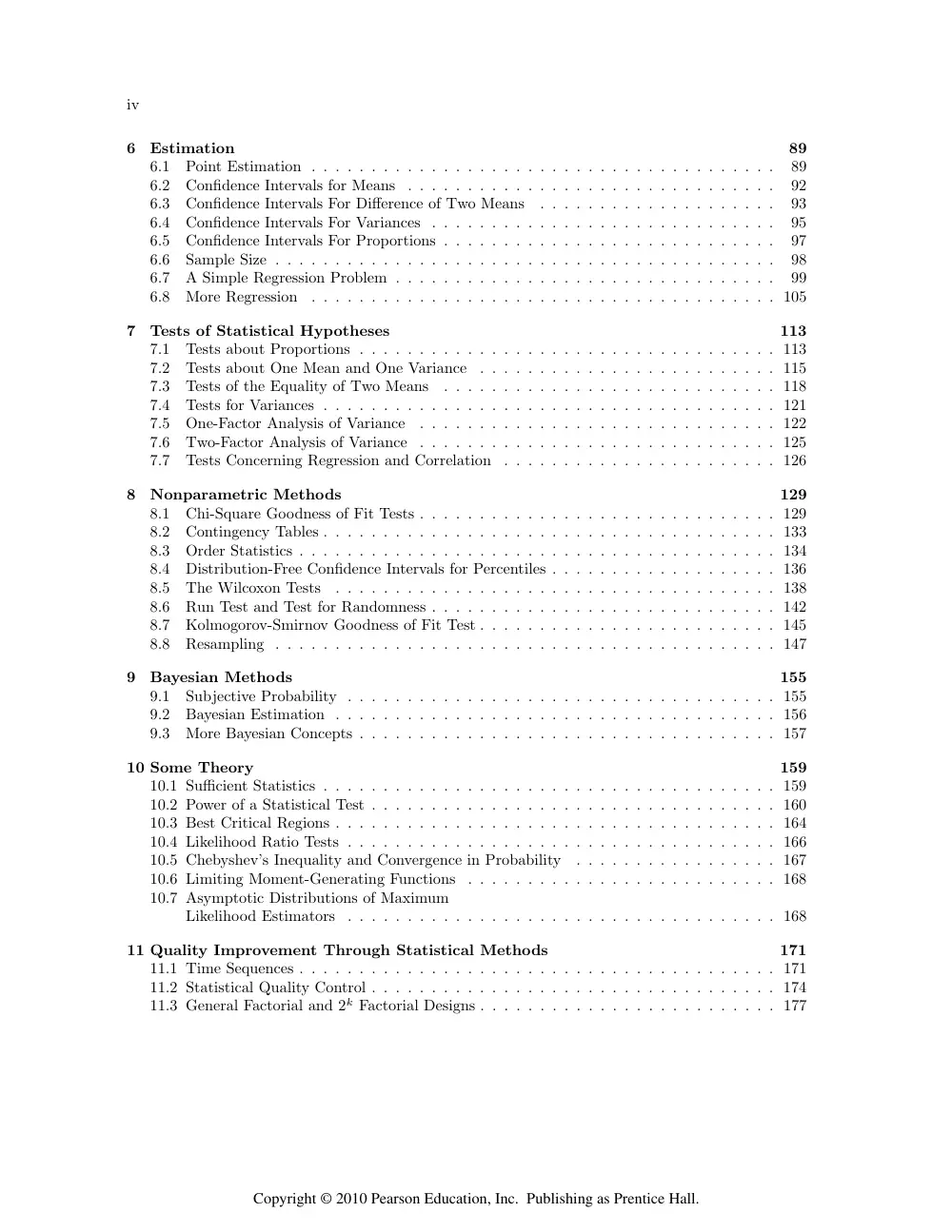iv 6 Estimation 89 6.1 Point Estimation . . . . . . . . . . . . . . . . . . . . . . . . . . . . . . . . . . . . . . . 89 6.2 Confidence Intervals for Means . . . . . . . . . . . . . . . . . . . . . . . . . . . . . . . 92 6.3 Confidence Intervals For Difference of Two Means . . . . . . . . . . . . . . . . . . . . 93 6.4 Confidence Intervals For Variances . . . . . . . . . . . . . . . . . . . . . . . . . . . . . 95 6.5 Confidence Intervals For Proportions . . . . . . . . . . . . . . . . . . . . . . . . . . . . 97 6.6 Sample Size . . . . . . . . . . . . . . . . . . . . . . . . . . . . . . . . . . . . . . . . . . 98 6.7 A Simple Regression Problem . . . . . . . . . . . . . . . . . . . . . . . . . . . . . . . . 99 6.8 More Regression . . . . . . . . . . . . . . . . . . . . . . . . . . . . . . . . . . . . . . . 105 7 Tests of Statistical Hypotheses 113 7.1 Tests about Proportions . . . . . . . . . . . . . . . . . . . . . . . . . . . . . . . . . . . 113 7.2 Tests about One Mean and One Variance . . . . . . . . . . . . . . . . . . . . . . . . . 115 7.3 Tests of the Equality of Two Means . . . . . . . . . . . . . . . . . . . . . . . . . . . . 118 7.4 Tests for Variances . . . . . . . . . . . . . . . . . . . . . . . . . . . . . . . . . . . . . . 121 7.5 One-Factor Analysis of Variance . . . . . . . . . . . . . . . . . . . . . . . . . . . . . . 122 7.6 Two-Factor Analysis of Variance . . . . . . . . . . . . . . . . . . . . . . . . . . . . . . 125 7.7 Tests Concerning Regression and Correlation . . . . . . . . . . . . . . . . . . . . . . . 126 8 Nonparametric Methods 129 8.1 Chi-Square Goodness of Fit Tests . . . . . . . . . . . . . . . . . . . . . . . . . . . . . . 129 8.2 Contingency Tables . . . . . . . . . . . . . . . . . . . . . . . . . . . . . . . . . . . . . . 133 8.3 Order Statistics . . . . . . . . . . . . . . . . . . . . . . . . . . . . . . . . . . . . . . . . 134 8.4 Distribution-Free Confidence Intervals for Percentiles . . . . . . . . . . . . . . . . . . . 136 8.5 The Wilcoxon Tests . . . . . . . . . . . . . . . . . . . . . . . . . . . . . . . . . . . . . 138 8.6 Run Test and Test for Randomness . . . . . . . . . . . . . . . . . . . . . . . . . . . . . 142 8.7 Kolmogorov-Smirnov Goodness of Fit Test . . . . . . . . . . . . . . . . . . . . . . . . . 145 8.8 Resampling . . . . . . . . . . . . . . . . . . . . . . . . . . . . . . . . . . . . . . . . . . 147 9 Bayesian Methods 155 9.1 Subjective Probability . . . . . . . . . . . . . . . . . . . . . . . . . . . . . . . . . . . . 155 9.2 Bayesian Estimation . . . . . . . . . . . . . . . . . . . . . . . . . . . . . . . . . . . . . 156 9.3 More Bayesian Concepts . . . . . . . . . . . . . . . . . . . . . . . . . . . . . . . . . . . 157 10 Some Theory 159 10.1 Sufficient Statistics . . . . . . . . . . . . . . . . . . . . . . . . . . . . . . . . . . . . . . 159 10.2 Power of a Statistical Test . . . . . . . . . . . . . . . . . . . . . . . . . . . . . . . . . . 160 10.3 Best Critical Regions . . . . . . . . . . . . . . . . . . . . . . . . . . . . . . . . . . . . . 164 10.4 Likelihood Ratio Tests . . . . . . . . . . . . . . . . . . . . . . . . . . . . . . . . . . . . 166 10.5 Chebyshev’s Inequality and Convergence in Probability . . . . . . . . . . . . . . . . . 167 10.6 Limiting Moment-Generating Functions . . . . . . . . . . . . . . . . . . . . . . . . . . 168 10.7 Asymptotic Distributions of Maximum Likelihood Estimators . . . . . . . . . . . . . . . . . . . . . . . . . . . . . . . . . . . . 168 11 Quality Improvement Through Statistical Methods 171 11.1 Time Sequences . . . . . . . . . . . . . . . . . . . . . . . . . . . . . . . . . . . . . . . . 171 11.2 Statistical Quality Control . . . . . . . . . . . . . . . . . . . . . . . . . . . . . . . . . . 174 11.3 General Factorial and 2k Factorial Designs . . . . . . . . . . . . . . . . . . . . . . . . . 177 Copyright © 2010 Pearson Education, Inc. Publishing as Prentice Hall. Preface This solutions manual provides answers for the even-numbered exercises in Probability and Statistical Inference, 8th edition, by Robert V. Hogg and Elliot A. Tanis. Complete solutions are given for most of these exercises. You, the instructor, may decide how many of these answers you want to make available to your students. Note that the answers for the odd-numbered exercises are given in the textbook. All of the figures in this manual were generated using Maple, a computer algebra system. Most of the figures were generated and many of the solutions, especially those involving data, were solved using procedures that were written by Zaven Karian from Denison University. We thank him for providing these. These procedures are available free of charge for your use. They are available on the CD-ROM in the textbook. Short descriptions of these procedures are provided on the “Maple Card” on the CD-ROM. Complete descriptions of these procedures are given in Probability and Statistics: Explorations with MAPLE, second edition, 1999, written by Zaven Karian and Elliot Tanis, published by Prentice Hall (ISBN 0-13-021536-8). Our hope is that this solutions manual will be helpful to each of you in your teaching. If you find an error or wish to make a suggestion, send these to Elliot Tanis at tanis@hope.edu and he will post corrections on his web page, http://www.math.hope.edu/tanis/. R.V.H. E.A.T. v Copyright © 2010 Pearson Education, Inc. Publishing as Prentice Hall. Chapter 1 Probability 1.1 Basic Concepts 1.1-2 (a) S = {bbb, gbb, bgb, bbg, bgg, gbg, ggb, ggg}; (b) S = {female, male}; (c) S = {000, 001, 002, 003, . . . , 999}. 1.1-4 (a) Clutch size: 4 5 6 7 8 9 10 11 12 13 14 Frequency: 3 5 7 27 26 37 8 2 0 1 1 (b) x h(x) 0.05 0.10 0.15 0.20 0.25 0.30 2 4 6 8 10 12 14 Figure 1.1–4: Clutch sizes for the common gallinule (c) 9. 1 Copyright © 2010 Pearson Education, Inc. Publishing as Prentice Hall. 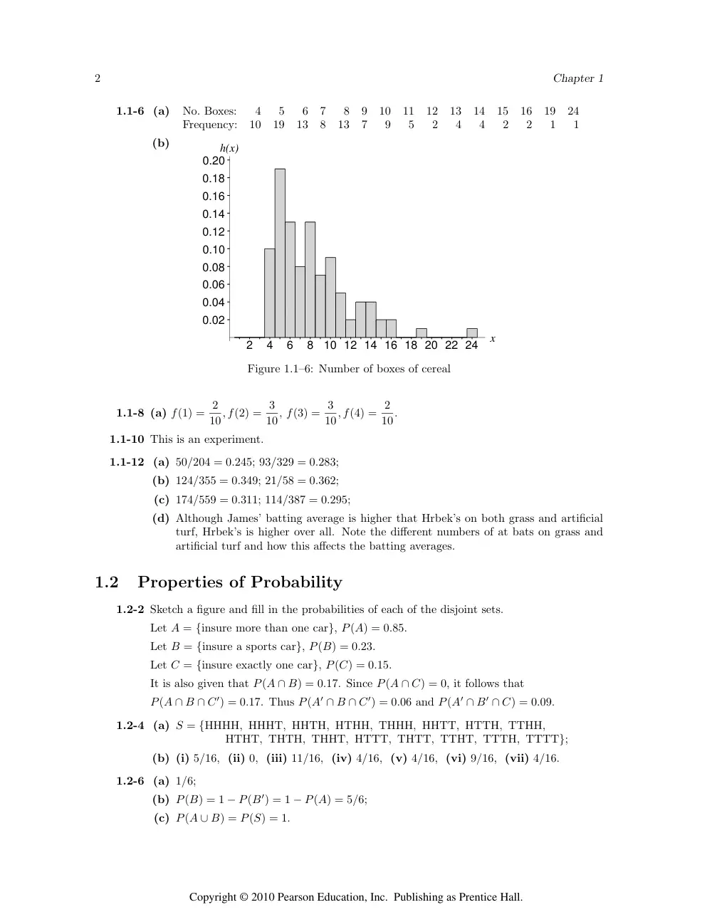2 Chapter 1 1.1-6 (a) No. Boxes: 4 5 6 7 8 9 10 11 12 13 14 15 16 19 24 Frequency: 10 19 13 8 13 7 9 5 2 4 4 2 2 1 1 (b) x h(x) 0.02 0.04 0.06 0.08 0.10 0.12 0.14 0.16 0.18 0.20 2 4 6 8 10 12 14 16 18 20 22 24 Figure 1.1–6: Number of boxes of cereal 1.1-8 (a) f(1) = 2 10, f(2) = 3 10, f(3) = 3 10, f(4) = 2 10. 1.1-10 This is an experiment. 1.1-12 (a) 50/204 = 0.245; 93/329 = 0.283; (b) 124/355 = 0.349; 21/58 = 0.362; (c) 174/559 = 0.311; 114/387 = 0.295; (d) Although James’ batting average is higher that Hrbek’s on both grass and artificial turf, Hrbek’s is higher over all. Note the different numbers of at bats on grass and artificial turf and how this affects the batting averages. 1.2 Properties of Probability 1.2-2 Sketch a figure and fill in the probabilities of each of the disjoint sets. Let A = {insure more than one car}, P(A) = 0.85. Let B = {insure a sports car}, P(B) = 0.23. Let C = {insure exactly one car}, P(C) = 0.15. It is also given that P(A ∩ B) = 0.17. Since P(A ∩ C) = 0, it follows that P(A ∩ B ∩ C′) = 0.17. Thus P(A′ ∩ B ∩ C′) = 0.06 and P(A′ ∩ B′ ∩ C) = 0.09. 1.2-4 (a) S = {HHHH, HHHT, HHTH, HTHH, THHH, HHTT, HTTH, TTHH, HTHT, THTH, THHT, HTTT, THTT, TTHT, TTTH, TTTT}; (b) (i) 5/16, (ii) 0, (iii) 11/16, (iv) 4/16, (v) 4/16, (vi) 9/16, (vii) 4/16. 1.2-6 (a) 1/6; (b) P(B) = 1 − P(B′) = 1 − P(A) = 5/6; (c) P(A ∪ B) = P(S) = 1. Copyright © 2010 Pearson Education, Inc. Publishing as Prentice Hall. Probability 3 1.2-8 (a) P(A ∪ B) = 0.4 + 0.5 − 0.3 = 0.6; (b) A = (A ∩ B′) ∪ (A ∩ B) P(A) = P(A ∩ B′) + P(A ∩ B) 0.4 = P(A ∩ B′) + 0.3 P(A ∩ B) = 0.1; (c) P(A′ ∪ B′) = P[(A ∩ B)′] = 1 − P(A ∩ B) = 1 − 0.3 = 0.7. 1.2-10 Let A ={lab work done}, B ={referral to a specialist}, P(A) = 0.41, P(B) = 0.53, P([A ∪ B]′) = 0.21. P(A ∪ B) = P(A) + P(B) − P(A ∩ B) 0.79 = 0.41 + 0.53 − P(A ∩ B) P(A ∩ B) = 0.41 + 0.53 − 0.79 = 0.15. 1.2-12 A ∪ B ∪ C = A ∪ (B ∪ C) P(A ∪ B ∪ C) = P(A) + P(B ∪ C) − P[A ∩ (B ∪ C)] = P(A) + P(B) + P(C) − P(B ∩ C) − P[(A ∩ B) ∪ (A ∩ C)] = P(A) + P(B) + P(C) − P(B ∩ C) − P(A ∩ B) − P(A ∩ C) + P(A ∩ B ∩ C). 1.2-14 (a) 1/3; (b) 2/3; (c) 0; (d) 1/2. 1.2-16 (a) S = {(1, 2), (1, 3), (1, 4), (1, 5), (2, 3), (2, 4), (2, 5), (3, 4), (3, 5), (4, 5)}; (b) (i) 1/10; (ii) 5/10. 1.2-18 P(A) = 2[r − r( √ 3/2)] 2r = 1 − √ 3 2 . 1.2-20 Note that the respective probabilities are p0, p1 = p0/4, p2 = p0/42, . . .. ∞ � k=0 p0 4k = 1 p0 1 − 1/4 = 1 p0 = 3 4 1 − p0 − p1 = 1 − 15 16 = 1 16. 1.3 Methods of Enumeration 1.3-2 (4)(3)(2) = 24. 1.3-4 (a) (4)(5)(2) = 40; (b) (2)(2)(2) = 8. 1.3-6 (a) 4 �6 3 � = 80; (b) 4(26) = 256; (c) (4 − 1 + 3)! (4 − 1)!3! = 20. 1.3-8 9P4 = 9! 5! = 3024. Copyright © 2010 Pearson Education, Inc. Publishing as Prentice Hall. 4 Chapter 1 1.3-10 S ={ HHH, HHCH, HCHH, CHHH, HHCCH, HCHCH, CHHCH, HCCHH, CHCHH, CCHHH, CCC, CCHC, CHCC, HCCC, CCHHC, CHCHC, HCCHC, CHHCC, HCHCC, HHCCC } so there are 20 possibilities. 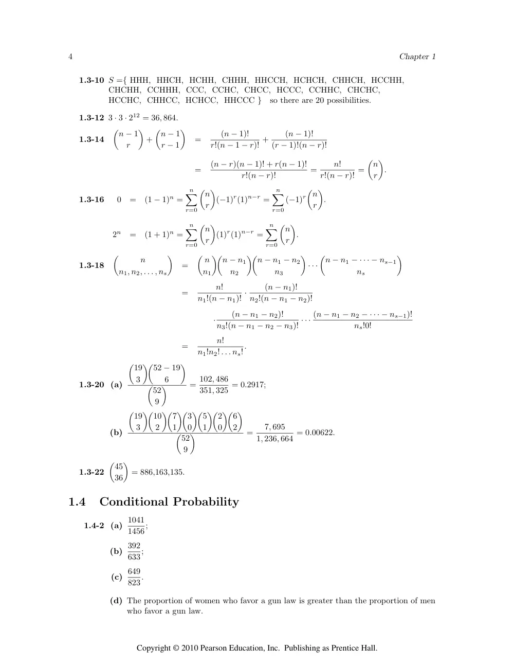1.3-12 3 · 3 · 212 = 36, 864. 1.3-14 �n − 1 r � + �n − 1 r − 1 � = (n − 1)! r!(n − 1 − r)! + (n − 1)! (r − 1)!(n − r)! = (n − r)(n − 1)! + r(n − 1)! r!(n − r)! = n! r!(n − r)! = �n r � . 1.3-16 0 = (1 − 1)n = n � r=0 �n r � (−1)r(1)n−r = n � r=0 (−1)r �n r � . 2n = (1 + 1)n = n � r=0 �n r � (1)r(1)n−r = n � r=0 �n r � . 1.3-18 � n n1, n2, . . . , ns � = � n n1 ��n − n1 n2 ��n − n1 − n2 n3 � · · · �n − n1 − · · · − ns−1 ns � = n! n1!(n − n1)! · (n − n1)! n2!(n − n1 − n2)! · (n − n1 − n2)! n3!(n − n1 − n2 − n3)! · · · (n − n1 − n2 − · · · − ns−1)! ns!0! = n! n1!n2! . . . ns!. 1.3-20 (a) �19 3 ��52 − 19 6 � �52 9 � = 102, 486 351, 325 = 0.2917; (b) �19 3 ��10 2 ��7 1 ��3 0 ��5 1 ��2 0 ��6 2 � �52 9 � = 7, 695 1, 236, 664 = 0.00622. 1.3-22 �45 36 � = 886,163,135. 1.4 Conditional Probability 1.4-2 (a) 1041 1456; (b) 392 633; (c) 649 823. (d) The proportion of women who favor a gun law is greater than the proportion of men who favor a gun law. Copyright © 2010 Pearson Education, Inc. Publishing as Prentice Hall. 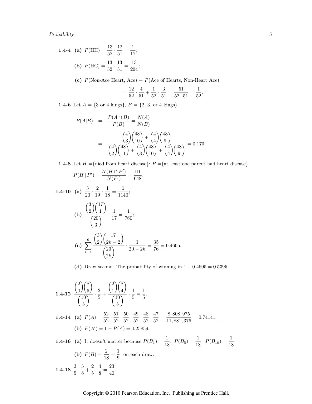Probability 5 1.4-4 (a) P(HH) = 13 52 · 12 51 = 1 17; (b) P(HC) = 13 52 · 13 51 = 13 204; (c) P(Non-Ace Heart, Ace) + P(Ace of Hearts, Non-Heart Ace) = 12 52 · 4 51 + 1 52 · 3 51 = 51 52 · 51 = 1 52. 1.4-6 Let A = {3 or 4 kings}, B = {2, 3, or 4 kings}. P(A|B) = P(A ∩ B) P(B) = N(A) N(B) = �4 3 ��48 10 � + �4 4 ��48 9 � �4 2 ��48 11 � + �4 3 ��48 10 � + �4 4 ��48 9 � = 0.170. 1.4-8 Let H ={died from heart disease}; P ={at least one parent had heart disease}. P(H | P ′) = N(H ∩ P ′) N(P ′) = 110 648. 1.4-10 (a) 3 20 · 2 19 · 1 18 = 1 1140; (b) �3 2 ��17 1 � �20 3 � · 1 17 = 1 760; (c) 9 � k=1 �3 2 �� 17 2k − 2 � �20 2k � · 1 20 − 2k = 35 76 = 0.4605. (d) Draw second. The probability of winning in 1 − 0.4605 = 0.5395. 1.4-12 �2 0 ��8 5 � �10 5 � · 2 5 + �2 1 ��8 4 � �10 5 � · 1 5 = 1 5. 1.4-14 (a) P(A) = 52 52 · 51 52 · 50 52 · 49 52 · 48 52 · 47 52 = 8, 808, 975 11, 881, 376 = 0.74141; (b) P(A′) = 1 − P(A) = 0.25859. 1.4-16 (a) It doesn’t matter because P(B1) = 1 18, P(B5) = 1 18, P(B18) = 1 18; (b) P(B) = 2 18 = 1 9 on each draw. 1.4-18 3 5 · 5 8 + 2 5 · 4 8 = 23 40. Copyright © 2010 Pearson Education, Inc. Publishing as Prentice Hall. 6 Chapter 1 1.4-20 (a) P(A1) = 30/100; (b) P(A3 ∩ B2) = 9/100; (c) P(A2 ∪ B3) = 41/100 + 28/100 − 9/100 = 60/100; (d) P(A1 | B2) = 11/41; (e) P(B1 | A3) = 13/29. 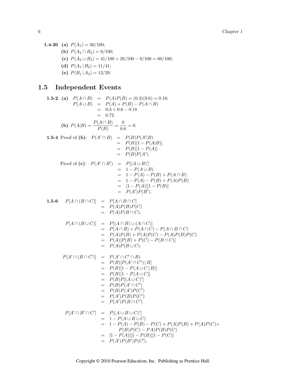1.5 Independent Events 1.5-2 (a) P(A ∩ B) = P(A)P(B) = (0.3)(0.6) = 0.18; P(A ∪ B) = P(A) + P(B) − P(A ∩ B) = 0.3 + 0.6 − 0.18 = 0.72. (b) P(A|B) = P(A ∩ B) P(B) = 0 0.6 = 0. 1.5-4 Proof of (b): P(A′ ∩ B) = P(B)P(A′|B) = P(B)[1 − P(A|B)] = P(B)[1 − P(A)] = P(B)P(A′). Proof of (c): P(A′ ∩ B′) = P[(A ∪ B)′] = 1 − P(A ∪ B) = 1 − P(A) − P(B) + P(A ∩ B) = 1 − P(A) − P(B) + P(A)P(B) = [1 − P(A)][1 − P(B)] = P(A′)P(B′). 1.5-6 P[A ∩ (B ∩ C)] = P[A ∩ B ∩ C] = P(A)P(B)P(C) = P(A)P(B ∩ C). P[A ∩ (B ∪ C)] = P[(A ∩ B) ∪ (A ∩ C)] = P(A ∩ B) + P(A ∩ C) − P(A ∩ B ∩ C) = P(A)P(B) + P(A)P(C) − P(A)P(B)P(C) = P(A)[P(B) + P(C) − P(B ∩ C)] = P(A)P(B ∪ C). P[A′ ∩ (B ∩ C′)] = P(A′ ∩ C′ ∩ B) = P(B)[P(A′ ∩ C′) | B] = P(B)[1 − P(A ∪ C | B)] = P(B)[1 − P(A ∪ C)] = P(B)P[(A ∪ C)′] = P(B)P(A′ ∩ C′) = P(B)P(A′)P(C′) = P(A′)P(B)P(C′) = P(A′)P(B ∩ C′) P[A′ ∩ B′ ∩ C′] = P[(A ∪ B ∪ C)′] = 1 − P(A ∪ B ∪ C) = 1 − P(A) − P(B) − P(C) + P(A)P(B) + P(A)P(C)+ P(B)P(C) − PA)P(B)P(C) = [1 − P(A)][1 − P(B)][1 − P(C)] = P(A′)P(B′)P(C′). Copyright © 2010 Pearson Education, Inc. Publishing as Prentice Hall. Probability 7 1.5-8 1 6 · 2 6 · 3 6 + 1 6 · 4 6 · 3 6 + 5 6 · 2 6 · 3 6 = 2 9. 1.5-10 (a) 3 4 · 3 4 = 9 16; (b) 1 4 · 3 4 + 3 4 · 2 4 = 9 16; (c) 2 4 · 1 4 + 2 4 · 4 4 = 10 16. 1.5-12 (a) �1 2 �3�1 2 �2 ; (b) �1 2 �3�1 2 �2 ; (c) �1 2 �3�1 2 �2 ; (d) 5! 3! 2! �1 2 �3�1 2 �2 . 1.5-14 (a) 1 − (0.4)3 = 1 − 0.064 = 0.936; (b) 1 − (0.4)8 = 1 − 0.00065536 = 0.99934464. 1.5-16 (a) ∞ � k=0 1 5 �4 5 �2k = 5 9; (b) 1 5 + 4 5 · 3 4 · 1 3 + 4 5 · 3 4 · 2 3 · 1 2 · 1 1 = 3 5. 1.5-18 (a) 7; (b) (1/2)7; (c) 63; (d) No! (1/2)63 = 1/9,223,372,036,854,775,808. 1.5-20 n 3 6 9 12 15 (a) 0.7037 0.6651 0.6536 0.6480 0.6447 (b) 0.6667 0.6319 0.6321 0.6321 0.6321 (c) Very little when n > 15, sampling with replacement Very little when n > 10, sampling without replacement. (d) Convergence is faster when sampling with replacement. 1.6 Bayes’s Theorem 1.6-2 (a) P(G) = P(A ∩ G) + P(B ∩ G) = P(A)P(G | A) + P(B)P(G | B) = (0.40)(0.85) + (0.60)(0.75) = 0.79; (b) P(A | G) = P(A ∩ G) P(G) = (0.40)(0.85) 0.79 = 0.43. Copyright © 2010 Pearson Education, Inc. Publishing as Prentice Hall. 8 Chapter 1 1.6-4 Let event B denote an accident and let A1 be the event that age of the driver is 16–25. Then P(A1 | B) = (0.1)(0.05) (0.1)(0.05) + (0.55)(0.02) + (0.20)(0.03) + (0.15)(0.04) = 50 50 + 110 + 60 + 60 = 50 280 = 0.179. 1.6-6 Let B be the event that the policyholder dies. Let A1, A2, A3 be the events that the deceased is standard, preferred and ultra-preferred, respectively. Then P(A1 | B) = (0.60)(0.01) (0.60)(0.01) + (0.30)(0.008) + (0.10)(0.007) = 60 60 + 24 + 7 = 60 91 = 0.659; P(A2 | B) = 24 91 = 0.264; P(A3 | B) = 7 91 = 0.077. 1.6-8 Let A be the event that the DVD player is under warranty. P(B1 | A) = (0.40)(0.10) (0.40)(0.10) + (0.30)(0.05) + (0.20)(0.03) + (0.10)(0.02) = 40 40 + 15 + 6 + 2 = 40 63 = 0.635; P(B2 | A) = 15 63 = 0.238; P(B3 | A) = 6 63 = 0.095; P(B4 | A) = 2 63 = 0.032. 1.6-10 (a) P(AD) = (0.02)(0.92) + (0.98)(0.05) = 0.0184 + 0.0490 = 0.0674; (b) P(N | AD) = 0.0490 0.0674 = 0.727; P(A | AD) = 0.0184 0.0674 = 0.273; (c) P(N | ND) = (0.98)(0.95) (0.02)(0.08) + (0.98)(0.95) = 9310 16 + 9310 = 0.998; P(A | ND) = 0.002. (d) Yes, particularly those in part (b). 1.6-12 Let D = {has the disease}, DP ={detects presence of disease}. Then P(D | DP) = P(D ∩ DP) P(DP) = P(D) · P(DP | D) P(D) · P(DP | D) + P(D′) · P(DP | D′) = (0.005)(0.90) (0.005)(0.90) + (0.995)(0.02) = 0.0045 0.0045 + 0.199 = 0.0045 0.0244 = 0.1844. Copyright © 2010 Pearson Education, Inc. Publishing as Prentice Hall. Probability 9 1.6-14 Let D = {defective roll} Then P(I | D) = P(I ∩ D) P(D) = P(I) · P(D | I) P(I) · P(D | I) + P(II) · P(D | II) = (0.60)(0.03) (0.60)(0.03) + (0.40)(0.01) = 0.018 0.018 + 0.004 = 0.018 0.022 = 0.818. Copyright © 2010 Pearson Education, Inc. Publishing as Prentice Hall. Chapter 2 Discrete Distributions 2.1 Random Variables of the Discrete Type 2.1-2 (a) f(x) =    0.6, x = 1, 0.3, x = 5, 0.1, x = 10, (b) f(x) x 0.1 0.2 0.3 0.4 0.5 0.6 1 2 3 4 5 6 7 8 9 10 Figure 2.1–2: A probability histogram 2.1-4 (a) f(x) = 1 10 , x = 0, 1, 2, · · · , 10; (b) N({0})/150 = 11/150 = 0.073; N({5})/150 = 13/150 = 0.087; N({1})/150 = 14/150 = 0.093; N({6})/150 = 22/150 = 0.147; N({2})/150 = 13/150 = 0.087; N({7})/150 = 16/150 = 0.107; N({3})/150 = 12/150 = 0.080; N({8})/150 = 18/150 = 0.120; N({4})/150 = 16/150 = 0.107; N({9})/150 = 15/150 = 0.100. 11 Copyright © 2010 Pearson Education, Inc. Publishing as Prentice Hall. 12 Chapter 2 (c) x f(x), h(x) 0.02 0.04 0.06 0.08 0.10 0.12 0.14 1 2 3 4 5 6 7 8 9 Figure 2.1–4: Michigan daily lottery digits 2.1-6 (a) f(x) = 6 − | 7 − x | 36 , x = 2, 3, 4, 5, 6, 7, 8, 9, 10, 11, 12. (b) x f(x) 0.02 0.04 0.06 0.08 0.10 0.12 0.14 0.16 1 2 3 4 5 6 7 8 9 10 11 12 Figure 2.1–6: Probability histogram for the sum of a pair of dice Copyright © 2010 Pearson Education, Inc. Publishing as Prentice Hall. Discrete Distributions 13 2.1-8 (a) The space of W is S = {0, 1, 2, 3, 4, 5, 6, 7}. P(W = 0) = P(X = 0, Y = 0) = 1 2 · 1 4 = 1 8, assuming independence. P(W = 1) = P(X = 0, Y = 1) = 1 2 · 1 4 = 1 8, P(W = 2) = P(X = 2, Y = 0) = 1 2 · 1 4 = 1 8, P(W = 3) = P(X = 2, Y = 1) = 1 2 · 1 4 = 1 8, P(W = 4) = P(X = 0, Y = 4) = 1 2 · 1 4 = 1 8, P(W = 5) = P(X = 0, Y = 5) = 1 2 · 1 4 = 1 8, P(W = 6) = P(X = 2, Y = 4) = 1 2 · 1 4 = 1 8, P(W = 7) = P(X = 2, Y = 5) = 1 2 · 1 4 = 1 8. That is, f(w) = P(W = w) = 1 8, w ∈ S. (b) x ( ) f x 0.02 0.04 0.06 0.08 0.10 0.12 1 2 3 4 5 6 7 Figure 2.1–8: Probability histogram of sum of two special dice 2.1-10 (a) �3 1 ��47 9 � �50 10 � = 39 98; (b) 1 � x=0 �3 x �� 47 10 − x � �50 10 � = 221 245. Copyright © 2010 Pearson Education, Inc. Publishing as Prentice Hall. 14 Chapter 2 2.1-12 OC(0.04) = �1 0 ��24 5 � �25 5 � + �1 1 ��24 4 � �25 5 � = 1.000; OC(0.08) = �2 0 ��23 5 � �25 5 � + �2 1 ��23 4 � �25 5 � = 0.967; OC(0.12) = �3 0 ��22 5 � �25 5 � + �3 1 ��22 4 � �25 5 � = 0.909; OC(0.16) = �4 0 ��21 5 � �25 5 � + �4 1 ��21 4 � �25 5 � = 0.834. 2.1-14 P(X ≥ 1) = 1 − P(X = 0) = 1 − �3 0 ��17 5 � �20 5 � = 1 − 91 228 = 137 228 = 0.60. 2.1-16 (a) Let Y equal the number of H chips that are selected. Then X = |Y − (10 − Y )| = |2Y − 10| and the p.m.f. of Y is g(y) = �10 y �� 10 10 − y � �20 10 � , y = 0, 1, . . . , 10. The p.m.f. of X is as follows: f(0) = g(5) f(2) = 2g(6) f(4) = 2g(7) f(6) = 2g(8) f(8) = 2g(9) f(10) = 2g(10) 1 184,756 2025 92,378 22,050 46,189 22,050 46,189 2025 92,378 1 92,378 (b) The mode is equal to 2. 2.1-18 (a) P(2, 1, 6, 10) means that 2 is in position 1 so 1 cannot be selected. Thus P(2, 1, 6, 10) = �1 0 ��1 1 ��8 5 � �10 6 � = 56 210 = 4 15; (b) P(i, r, k, n) = �i − 1 r − 1 ��1 1 ��n − i k − r � �n k � . Copyright © 2010 Pearson Education, Inc. Publishing as Prentice Hall. Discrete Distributions 15 2.2 Mathematical Expectation 2.2-2 E(X) = (−1) �4 9 � + (0) �1 9 � + (1) �4 9 � = 0; E(X2) = (−1)2 �4 9 � + (0)2 �1 9 � + (1)2 �4 9 � = 8 9; E(3X2 − 2X + 4) = 3 �8 9 � − 2(0) + 4 = 20 3 . 2.2-4 E(X) = $ 499(0.001) − $ 1(0.999) = −$ 0.50. 2.2-6 1 = 6 � x=0 f(x) = 9 10 + c �1 1 + 1 2 + 1 3 + 1 4 + 1 5 + 1 6 � c = 2 49; E(Payment) = 2 49 � 1 · 1 2 + 2 · 1 3 + 3 · 1 4 + 4 · 1 5 + 5 · 1 6 � = 71 490 units. 2.2-8 Note that ∞ � x=1 6 π2x2 = 6 π2 ∞ � x=1 1 x2 = 6 π2 π2 6 = 1, so this is a p.d.f. E(X) = ∞ � x=1 x 6 π2x2 = 6 π2 ∞ � x=1 1 x and it is well known that the sum of this harmonic series is not finite. 2.2-10 E(|X − c|) = 1 7 � x∈S |x − c|, where S = {1, 2, 3, 5, 15, 25, 50}. When c = 5, E(|X − 5|) = 1 7 [(5 − 1) + (5 − 2) + (5 − 3) + (5 − 5) + (15 − 5) + (25 − 5) + (50 − 5)] . If c is either increased or decreased by 1, this expectation is increased by 1/7. Thus c = 5, the median, minimizes this expectation while b = E(X) = µ, the mean, minimizes E[(X − b)2]. You could also let h(c) = E( | X − c | ) and show that h′(c) = 0 when c = 5. 2.2-12 (1) · 15 36 + (−1) · 21 36 = −6 36 = −1 6 ; (1) · 15 36 + (−1) · 21 36 = −6 36 = −1 6 ; (4) · 6 36 + (−1) · 30 36 = −6 36 = −1 6 . 2.2-14 (a) The average class size is (16)(25) + (3)(100) + (1)(300) 20 = 50; (b) f(x) =    0.4, x = 25, 0.3, x = 100, 0.3, x = 300, (c) E(X) = 25(0.4) + 100(0.3) + 300(0.3) = 130. Copyright © 2010 Pearson Education, Inc. Publishing as Prentice Hall. 16 Chapter 2 2.3 The Mean, Variance, and Standard Deviation 2.3-2 (a) µ = E(X) = 3 � x=1 x 3! x! (3 − x)! �1 4 �x�3 4 �3−x = 3 �1 4 � 2 � k=0 2! k! (2 − k)! �1 4 �k�3 4 �2−k = 3 �1 4 ��1 4 + 3 4 �2 = 3 4; E[X(X − 1)] = 3 � x=2 x(x − 1) 3! x! (3 − x)! �1 4 �x�3 4 �3−x = 2(3) �1 4 �2 3 4 + 6 �1 4 �3 = 6 �1 4 �2 = 2 �1 4 ��3 4 � ; σ2 = E[X(X − 1)] + E(X) − µ2 = (2) �3 4 ��1 4 � + �3 4 � − �3 4 �2 = (2) �3 4 ��1 4 � + �3 4 ��1 4 � = 3 �1 4 ��3 4 � ; (b) µ = E(X) = 4 � x=1 x 4! x! (4 − x)! �1 2 �x�1 2 �4−x = 4 �1 2 � 3 � k=0 3! k! (3 − k)! �1 2 �k�1 2 �3−k = 4 �1 2 ��1 2 + 1 2 �3 = 2; E[X(X − 1)] = 4 � x=2 x(x − 1) 4! x! (4 − x)! �1 2 �x�1 2 �4−x = 2(6) �1 2 �4 + (6)(4) �1 2 �4 + (12) �1 2 �4 = 48 �1 2 �4 = 12 �1 2 �2 ; σ2 = (12) �1 2 �2 + 4 2 − �4 2 �2 = 1. 2.3-4 E[(X − µ)/σ] = (1/σ)[E(X) − µ] = (1/σ)(µ − µ) = 0; E{[(X − µ)/σ]2} = (1/σ2)E[(X − µ)2] = (1/σ2)(σ2) = 1. Copyright © 2010 Pearson Education, Inc. Publishing as Prentice Hall. Discrete Distributions 17 2.3-6 f(1) = 3 8, f(2) = 2 8, f(3) = 3 8 µ = 1 · 3 8 + 2 · 2 8 + 3 · 3 8 = 2, σ2 = 12 · 3 8 + 22 · 2 8 + 32 · 3 8 − 22 = 3 4. 2.3-8 (a) x = 4 3 = 1.333; (b) s2 = 88 69 = 1.275. 2.3-10 (a) [3, 19, 16, 9]; (b) x = 125 47 = 2.66, s = 0.87; (c) h(x) x 0.05 0.10 0.15 0.20 0.25 0.30 0.35 0.40 1 2 3 4 Figure 2.3–10: Number of pets 2.3-12 x = 409 50 = 8.18. 2.3-14 (a) f(x) = P(X = x) = �6 x �� 43 6 − x � �49 6 � , x = 0, 1, 2, 3, 4, 5, 6; (b) µX = 6 � x=0 xf(x) = 36 49 = 0.7347, σ2 X = 6 � x=0 (x − µ)2f(x) = 5,547 9,604 = 0.5776; σX = 43 98 √ 3 = 0.7600; (c) f(0) = 435,461 998,844 > 412,542 998,844 = f(1); X = 0 is most likely to occur. Copyright © 2010 Pearson Education, Inc. Publishing as Prentice Hall. 18 Chapter 2 (d) The numbers are reasonable because (25,000,000)f(6) = 1.79; (25,000,000)f(5) = 461.25; (25,000,000)f(4) = 24,215.49; (e) The respective expected values, (138)f(x), for x = 0, 1, 2, 3, are 60.16, 57.00, 18.27, and 2.44, so the results are reasonable. See Figure 2.3-14 for a comparison of the theoretical probability histogram and the histogram of the data. f(x), h(x) x 0.1 0.2 0.3 0.4 1 2 3 4 5 6 Figure 2.3–14: Empirical (shaded) and theoretical histograms for LOTTO 2.3-16 (a) Out of the 75 numbers, first select x − 1 of which 23 are selected out of the 24 good numbers on your card and the remaining x − 1 − 23 are selected out of the 51 bad numbers. There is now one good number to be selected out of the remaining 75 − (x − 1). (b) The mode is 75. (c) µ = 1824 25 = 72.96. (d) E[X(X + 1)] = 70,224 13 = 5,401.846154. (e) σ2 = 46,512 8,125 = 5.724554; σ = 2.3926. (f) (i) x = 72.78, (ii) s2 = 8.7187879, (iii) s = 2.9528, (iv) 5378.34. Copyright © 2010 Pearson Education, Inc. Publishing as Prentice Hall. Discrete Distributions 19 (g) x f(x), h(x) 0.05 0.10 0.15 0.20 0.25 0.30 0.35 61 63 65 67 69 71 73 75 Figure 2.3–16: Bingo “cover-up” comparisons 2.3-18 (a) P(X ≥ 1) = 21 �3 1 � = 2 3; (b) 5 � k=1 P(X ≥ k) = P(X = 1) + 2P(X = 2) + · · · + 5P(X = 5) = µ; (c) µ = 5,168 3,465 = 1.49149; (d) In the limit, µ = π 2 . 2.4 Bernoulli Trials and the Binomial Distribution 2.4-2 f(−1) = 11 18, f(1) = 7 18; µ = (−1)11 18 + (1) 7 18 = − 4 18; σ2 = � −1 + 4 18 �2�11 18 � + � 1 + 4 18 �2� 7 18 � = 77 81. 2.4-4 (a) P(X ≤ 5) = 0.6652; (b) P(X ≥ 6) = 1 − P(X ≤ 5) = 0.3348; (c) P(X ≤ 7) − P(X ≤ 6) = 0.9427 − 0.8418 = 0.1009; (d) µ = (12)(0.40) = 4.8, σ2 = (12)(0.40)(0.60) = 2.88, σ = √ 2.88 = 1.697. 2.4-6 (a) X is b(7, 0.15); (b) (i) P(X ≥ 2) = 1 − P(X ≤ 1) = 1 − 0.7166 = 0.2834; (ii) P(X = 1) = P(X ≤ 1) − P(X ≤ 0) = 0.7166 − 0.3206 = 0.3960; (iii) P(X ≤ 3) = 0.9879. Copyright © 2010 Pearson Education, Inc. Publishing as Prentice Hall. 20 Chapter 2 2.4-8 (a) P(X ≥ 10) = P(15 − X ≤ 5) = 0.5643; (b) P(X ≤ 10) = P(15 − X ≥ 5) = 1 − P(15 − X ≤ 4) = 1 − 0.3519 = 0.6481; (c) P(X = 10) = P(X ≥ 10) − P(X ≥ 11) = P(15 − X ≤ 5) − P(15 − X ≤ 4) = 0.5643 − 0.3519 = 0.2124; (d) X is b(15, 0.65), 15 − X) is b(15, 0.35); (e) µ = (15)(0.65) = 9.75, σ2 = (15)(0.65)(0.35) = 3.4125; σ = √ 3.4125 = 1.847. 2.4-10 (a) 1 − 0.014 = 0.99999999; (b) 0.994 = 0.960596. 2.4-12 (a) X is b(8, 0.90); (b) (i) P(X = 8) = P(8 − X = 0) = 0.4305; (ii) P(X ≤ 6) = P(8 − X ≥ 2) = 1 − P(8 − X ≤ 1) = 1 − 0.8131 = 0.1869; (iii) P(X ≥ 6) = P(8 − X ≤ 2) = 0.9619. 2.4-14 (a) f(x) =                125/216, x = −1, 75/216, x = 1, 15/216, x = 2, 1/216, x = 3; (b) µ = (−1) · 125 216 + (1) · 75 216 + (2) · 15 216 + (3) · 1 216 = − 17 216; σ2 = E(X2) − µ2 = 269 216 − � − 17 216 �2 = 1.2392; σ = 1.11; (c) See Figure 2.4-14. (d) x = −1 100 = −0.01; s2 = 100(129) − (−1)2 100(99) = 1.3029; s = 1.14. Copyright © 2010 Pearson Education, Inc. Publishing as Prentice Hall. Discrete Distributions 21 (e) f(x), h(x) x 0.1 0.2 0.3 0.4 0.5 –1 1 2 3 Figure 2.4–14: Losses in chuck-a-luck 2.4-16 Let X equal the number of winning tickets when n tickets are purchased. Then P(X ≥ 1) = 1 − P(X = 0) = 1 − � 9 10 �n . (a) 1 − (0.9)n = 0.50 (0.9)n = 0.50 n ln 0.9 = ln 0.5 n = ln 0.5 ln 0.9 = 6.58 so n = 7. (b) 1 − (0.9)n = 0.95 (0.9)n = 0.05 n = ln 0.05 ln 0.09 = 28.43 so n = 29. 2.4-18 (0.1)(1 − 0.955) (0.4)(1 − 0.975) + (0.5)(1 − 0.985) + (0.1)(1 − 0.955) = 0.178. 2.4-20 It is given that X is b(10, 0.10). We are to find M so that P(1000X ≤ M) ≥ 0.99) or P(X ≤ M/1000) ≥ 0.99. From Appendix Table II, P(X ≤ 4) = 0.9984 > 0.99. Thus M/1000 = 4 or M = 4000 dollars. 2.4-22 X is b(5, 0.05). The expected number of tests is 1 P(X = 0) + 6 P(X > 0) = 1 (0.7738) + 6 (1 − 0.7738) = 2.131. Copyright © 2010 Pearson Education, Inc. Publishing as Prentice Hall. 22 Chapter 2 2.5 The Moment-Generating Function 2.5-2 (a) (i) b(5, 0.7); (ii) µ = 3.5, σ2 = 1.05; (iii) 0.1607; (b) (i) geometric, p = 0.3; (ii) µ = 10/3, σ2 = 70/9; (iii) 0.51; (c) (i) Bernoulli, p = 0.55; (ii) µ = 0.55, σ2 = 0.2475; (iii) 0.55; (d) (ii) µ = 2.1, σ2 = 0.89; (iii) 0.7; (e) (i) negative binomial, p = 0.6, r = 2; (ii) 10/3, σ2 = 20/9; (iii) 0.36; (f) (i) discrete uniform on 1, 2, . . . , 10; (ii) 5.5, 8.25; (iii) 0.2. 2.5-4 (a) f(x) = �364 365 �x−1� 1 365 � , x = 1, 2, 3, . . . , (b) µ = 1 1 365 = 365, σ2 = 364 365 � 1 365 �2 = 132,860, σ = 364.500; (c) P(X > 400) = �364 365 �400 = 0.3337, P(X < 300) = 1 − �364 365 �299 = 0.5597. 2.5-6 P(X ≥ 100) = P(X > 99) = (0.99)99 = 0.3697. 2.5-8 �10 − 1 5 − 1 ��1 2 �5�1 2 �5 = 126 1024 = 63 512. 2.5-10 (a) Negative binomial with r = 10, p = 0.6 so µ = 10 0.60 = 16.667, σ2 = 10(0.40) (0.60)2 = 11.111, σ = 3.333; (b) P(X = 16) = �15 9 � (0.60)10(0.40)6 = 0.1240. 2.5-12 P(X > k + j | X > k) = P(X > k + j) P(X > k) = qk+j qk = qj = P(X > j). 2.5-14 (b) ∞ � x=2 f(x) = ∞ � x=2 1 √ 5   � 1 + √ 5 2 �x−1 − � 1 − √ 5 2 �x−1  � 1 2x � = 2 √ 5(1 + √ 5) ∞ � x=2 (1 + √ 5)x 4x − 2 √ 5(1 − √ 5) ∞ � x=2 (1 − √ 5)x 4x = (you fill in missing steps) = 1; Copyright © 2010 Pearson Education, Inc. Publishing as Prentice Hall. Discrete Distributions 23 (c) E(X) = ∞ � x=2 x √ 5   � 1 + √ 5 2 �x−1 − � 1 − √ 5 2 �x−1  � 1 2x � = 1 2 √ 5 ∞ � x=1  x � 1 + √ 5 4 �x−1 − x � 1 − √ 5 4 �x−1  = 1 2 √ 5 � 1 (1 − (1 + √ 5)/4)2 − 1 (1 − (1 − √ 5/4)2 � = (you fill in missing steps) = 6; (d) E[X(X − 1)] = ∞ � x=2 x(x − 1) 1 √ 5   � 1 + √ 5 2 �x−1 − � 1 − √ 5 2 �x−1  � 1 2x � = 1 2 √ 5 ∞ � x=2 x(x − 1)   � 1 + √ 5 4 �x−1 − � 1 − √ 5 4 �x−1  = 1 2 √ 5  1 + √ 5 4 ∞ � x=2 x(x − 1) � 1 + √ 5 4 �x−2 − 1 − √ 5 4 ∞ � x=2 x(x − 1) � 1 − √ 5 4 �x−2  = 1 2 √ 5   2 � 1 + √ 5 4 � � 1 − 1 + √ 5 4 �3 − 2 � 1 − √ 5 4 � � 1 − 1 − √ 5 4 �3   = (you fill in missing steps)