CSI 312 Lecture 2, Fall 2011

Computer Architecture Lecture 2 - Performance Fall 2011 Reading: 1.4 – 1.10 Homework: 1.3, 1.4, 1.5 Lecture 2 Performance- Abbas Tarhini (c) 2 Roadmap for the term: major topics Computer Systems Overview Technology Trends Instruction sets (and Software) Logic & Arithmetic Performance 3 Processor Implementation Memory Systems Input/Output Lecture 2 Performance- Abbas Tarhini (c) 3 Performance Outline Motivation 3 Defining Performance Common Performance Metrics Benchmarks Amdahl’s Law Lecture 2 Performance- Abbas Tarhini (c) 4 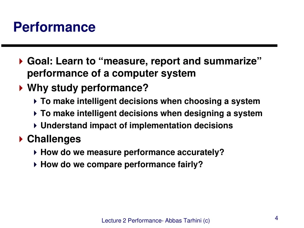Performance Goal: Learn to “measure, report and summarize” performance of a computer system Why study performance? To make intelligent decisions when choosing a system To make intelligent decisions when designing a system Understand impact of implementation decisions Challenges How do we measure performance accurately? How do we compare performance fairly? 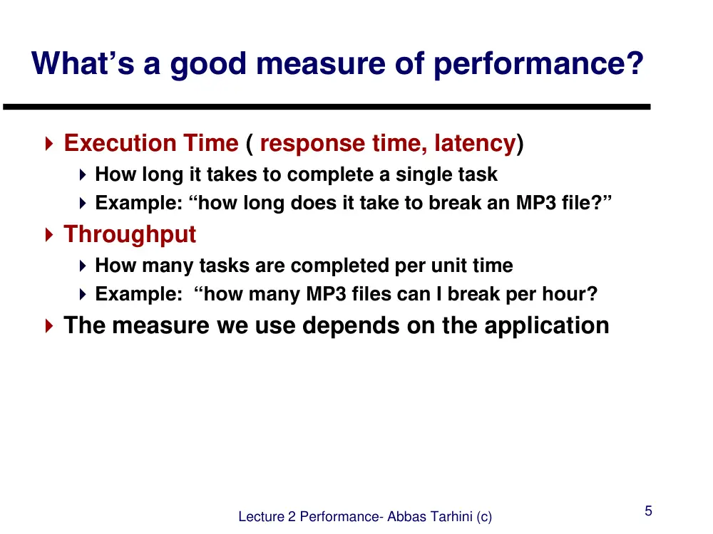Lecture 2 Performance- Abbas Tarhini (c) 5 What’s a good measure of performance? Execution Time ( response time, latency) How long it takes to complete a single task Example: “how long does it take to break an MP3 file?” Throughput How many tasks are completed per unit time Example: “how many MP3 files can I break per hour? 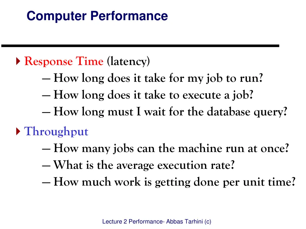The measure we use depends on the application Lecture 2 Performance- Abbas Tarhini (c) Response Time (latency) — How long does it take for my job to run? — How long does it take to execute a job? — How long must I wait for the database query? Throughput — How many jobs can the machine run at once? — What is the average execution rate? — How much work is getting done per unit time? 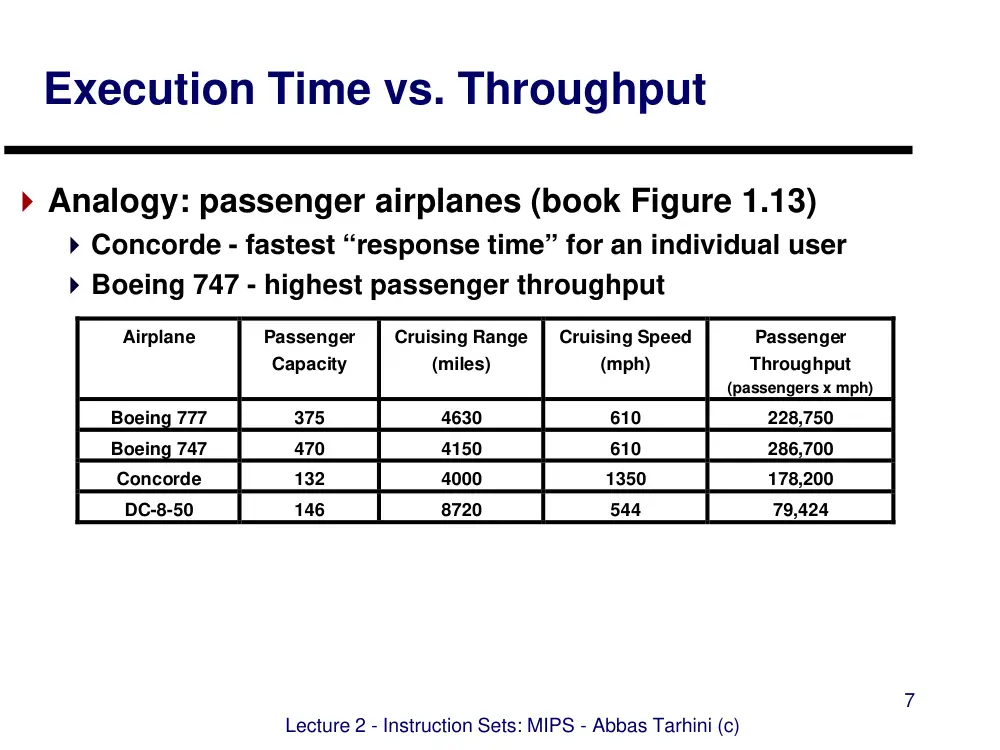Computer Performance Lecture 2 - Instruction Sets: MIPS - Abbas Tarhini (c) 7 Execution Time vs. Throughput Analogy: passenger airplanes (book Figure 1.13) Concorde - fastest “response time” for an individual user Boeing 747 - highest passenger throughput Airplane Passenger Capacity Cruising Range (miles) Cruising Speed (mph) Passenger Throughput (passengers x mph) Boeing 777 375 4630 610 228,750 Boeing 747 470 4150 610 286,700 Concorde 132 4000 1350 178,200 DC-8-50 146 8720 544 79,424 Lecture 2 Performance- Abbas Tarhini (c) 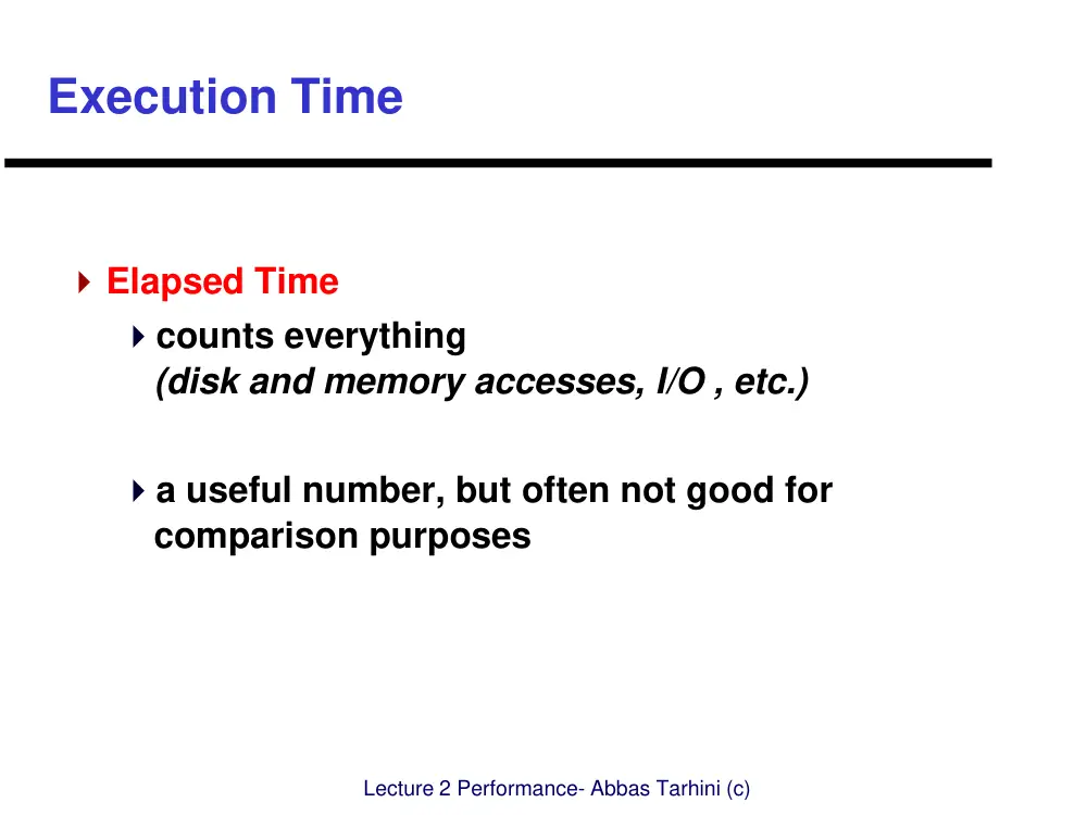Elapsed Time counts everything (disk and memory accesses, I/O , etc.) a useful number, but often not good for comparison purposes Execution Time Lecture 2 Performance- Abbas Tarhini (c) 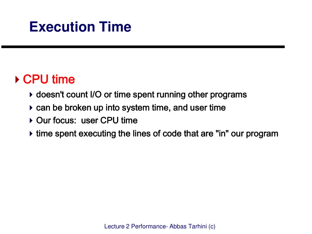Execution Time CPU time doesn't count I/O or time spent running other programs can be broken up into system time, and user time Our focus: user CPU time time spent executing the lines of code that are "in" our program Lecture 2 Performance- Abbas Tarhini (c) 10 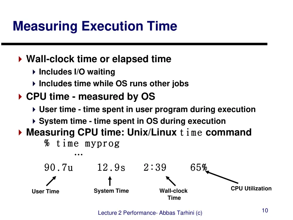Measuring Execution Time Wall-clock time or elapsed time Includes I/O waiting Includes time while OS runs other jobs CPU time - measured by OS User time - time spent in user program during execution System time - time spent in OS during execution Measuring CPU time: Unix/Linux time command % time myprog … 90.7u 12.9s 2:39 65% User Time System Time Wall-clock Time CPU Utilization Lecture 2 Performance- Abbas Tarhini (c) 11 Performance Outline Motivation Defining Performance 3 Common Performance Metrics Benchmarks Amdahl’s Law Lecture 2 Performance- Abbas Tarhini (c) 12 Defining Performance using Execution Time For a given program on machine X: Comparing performance of machines: PerformanceX > PerformanceY if Execution TimeX < Execution TimeY X X time Execution 1 Performance  Lecture 2 Performance- Abbas Tarhini (c) 13 Defining Performance (cont’d) We say “X is n times faster than Y” if: PerformanceX PerformanceY  n PerformanceX PerformanceY  Execution timeY Execution timeX  n Use this definition to compare performance in homework & exam problems! Lecture 2 Performance- Abbas Tarhini (c) 14 Example - Performance Which machine is faster? By how much? B A Machine Execution Time A 15 seconds B 20 seconds  n  PerformanceA PerformanceB  Execution timeB Execution timeA  20 sec. 15 sec. 1.33 A Lecture 2 Performance- Abbas Tarhini (c) 15 Performance Outline Motivation Defining Performance Common Performance Metrics 3 Benchmarks Amdahl’s Law Lecture 2 Performance- Abbas Tarhini (c) CPU Clocking Operation of digital hardware governed by a constant-rate clock Clock (cycles) Data transfer and computation Update state Clock period  Clock period: duration of a clock cycle  e.g., 250ps = 0.25ns = 250×10–12s  Clock frequency (rate): cycles per second  e.g., 4.0GHz = 4000MHz = 4.0×109Hz Lecture 2 Performance- Abbas Tarhini (c) 17 Clocks and Performance Every processor has a clock Clock frequency - MHz (or GHz) Clock cycle time / period - ns (or ps) How do we relate clock to program performance? Cycle time tclock= 2 ns fclk = 500 MHz 1 Hz means that an event repeats once per second cycle clock seconds program CPU time for a program = clock cycles  Clock cycle time CPU time for a program = # CPU clock cycle for a program x clock cycle time CPU time for a program = # CPU clock cycle for a program / clock rate. Clock cycle time = 1/clock rate Lecture 2 Performance- Abbas Tarhini (c) 18 Example - Clock Cycles How many clock cycles does A execute? How many clock cycles does B execute? Machine Execution Time Clock Freq. A 15 seconds 900 MHz B 20 seconds 600 MHz 15 seconds  900 106 cycles second  1.351010cycles 20 seconds  600 106 cycles second  1.21010 cycles CPU time for a program = CPU clock cycle for a program / clock rate. => CPU clock cycle for a program = CPU time for a program * clock rate Lecture 2 Performance- Abbas Tarhini (c) Consider a program that runs in 10 seconds on computer, A, which has a 4 GHZ clock. We are trying to help a computer designer build a computer, B, which will run this program in 6 seconds. The designer has determined that a substantial increase in the clock rate is possible, but this increase will affect the rest of the CPU design, causing computer B to require 1.2 times as many clock cycles as computer A for this program. What clock rate should we tell the designer to target? 19 Lecture 2 Performance- Abbas Tarhini (c) Answer: Performance equation First step: find clock cycles executed by Computer A 20 frequency clock cycles clock cycle clock onds sec program CPU time = clock cycles   second cycles 10 400 = 10 seconds = clock cycles Time CPU 6 A A  cycles 9 6 A 40 x 10 second cycles =10 seconds x 400 10 cycles clock   Lecture 2 Performance- Abbas Tarhini (c) 21 B 6 B rate Clock = 6seconds = 4800 10 cycles CPU Time  800MHz seconds 6 4800 10 cycles rate Clock 6 B    Answer: (continued) Second step: find clock cycles executed by Computer B Third step: given clock cycles and CPU time, solve for clock rate of Computer B 4800 106 cycles cycles clock 1.2 cycles clock A B     Lecture 2 Performance- Abbas Tarhini (c) 24 Clock Cycles per Instruction (CPI) Consider the following instructions ADDA - 3 cycles MUL - 10 cycles IDIV - 41 cycles More complex processors have other issues… Pipelining - parallel execution, but sometimes stalls Memory system issues: cache misses, page faults, etc. How can we combine these into an overall metric? add lda mul and sta Total Execution Time Lecture 2 Performance- Abbas Tarhini (c) 25 Definition: Clock Cycles per Instruction (CPI) Average number of clock cycles per instruction Measured for an entire program  => # of clock cycles = CPI * # of instructions.  => execution time = # of clock cycles / clock rate = CPI * # of instructions / clock rate. CPI  Average Cycles per Instruction = # of clock cycles # of instructions Lecture 2 Performance- Abbas Tarhini (c) 26 Example - CPI What is the CPI of A? What is the CPI of B? 1.351010cycles 2.6 109 instructions  5.2 Machine Clock Cycles Instructions A 1.35 X 1010 2.6 X 109 B 1.2 X 1010 3.0 X 109 1.2 1010 cycles 3.0 109 instructions  4.0 Lecture 2 Performance- Abbas Tarhini (c) 27 Definition - MIPS MIPS - millions of instructions per second Once used as a general metric for performance But, not useful for comparing different architectures Often ridiculed as “meaningless indicator of performance” MIPS  # of instructions benchmark program benchmark program execution time 1,000,000 Lecture 2 Performance- Abbas Tarhini (c) 28 Example - MIPS What is the MIPS of A? What is the MIPS of B? 2.6 109 instructions 15 seconds  1 MIPS 106 IPS 173.33 MIPS Machine Execution Time Instructions A 15 seconds 2.6 X 109 B 20 seconds 3.0 X 109 150 MIPS 3.0 109 instructions 20 seconds  1 MIPS 106 IPS Lecture 2 Performance- Abbas Tarhini (c) Assume an instruction set implemented in 2 architectures: For some program, Computer A has: clock cycle time = 250 ps CPI = 2.0 For the same program, Computer B has: clock cycle time = 500 ps CPI = 1.2 Which computer is faster? 29 Lecture 2 Performance- Abbas Tarhini (c) Answer: Computer A and B executes the same number of instructions for the program, let’s call it I. The number of clock cycles for each computer: CPU clock cycles for A = I x 2.0 CPU clock cycles for B = I x 1.2 CPU time for each computer: CPU time A = CPU clock cycles x Clock cycle time A = I x 2.0 x 250 ps = 500 x I ps CPU time B = CPU clock cycles x Clock cycle time B = I x 1.2 x 500 ps = 600 x I ps 30 Which is faster ? … Clearly A is faster: CPU performance A = Execution time B CPU performance B Execution time A = 600 x I ps = 1.2 times 500 x I ps Lecture 2 Performance- Abbas Tarhini (c) 31 Relating the Metrics - The Performance Equation CPU time = #instructions program  clock cycles instruction  seconds clock cycle The “Iron Law” of Performance: a complete and reliable measure of computer performance is time. So, to improve performance (everything else being equal) you can either increase or decrease? _decrease_ the # of required cycles for a program, or _decrease_ the clock cycle time or, said another way, _increase_ the clock rate. Lecture 2 Performance- Abbas Tarhini (c) 32 Self Test !: Clock Cycles and Performance - Example Program runs on Computer A: CPU Time: 10 seconds Clock: 400MHz Computer B can run clock faster But, requires 1.2X clock cycles to perform same task Desired CPU Time: 6 Seconds What should the clock frequency be to reach this target? Key to approach: Performance equation CPU time = clock cycles program  seconds clock cycle  clock cycles clock frequency Lecture 2 Performance- Abbas Tarhini (c) 33 Remember: CPU clock cycles = Instructions for a program x Average clock cycles per Instruction (CPI) CPU time = Instruction count x CPI x clock cycle time rate Clock CPI Instruction count CPU time   Lecture 2 - Instruction Sets: MIPS - Abbas Tarhini (c) 34 Basic measurment at different levels in the computer and what is measured: Components of Performance Units of Measure CPU execution time for a program Seconds for the program Instruction count Instructions executed for the program Clock Cycles per Instruction (CPI) Average number of clock cycles per instruction Clock cycle time Seconds per clock cycle Lecture 2 Performance- Abbas Tarhini (c) 35 CPUi : the average number of cycles per instructions for that instruction class Ci : the count of the number of instructions of class i executed. n : the number of instruction classes. More on CPU Clock Cycles ) ( clock cycles n 1 i i i C CPU CPU    If a program contains different type of instruction using different clock cycle counts, then Lecture 2 Performance- Abbas Tarhini (c) 36 Homework Instruction Classes: Add Multiply Average Clock Cycles per Instruction: Add 1 clock cycle Mul 3 clock cycles Program A executed: 10 Add instructions 5 Multiply instructions What is the CPU clock cycle times? What is the average CPI? Lecture 2 Performance- Abbas Tarhini (c) 37 Lecture 2 Performance- Abbas Tarhini (c) 38 Lecture 2 Performance- Abbas Tarhini (c) 39 Lecture 2 Performance- Abbas Tarhini (c) 40 Performance Tradeoffs Program Instruction count - impacted by Instructions available to perform basic tasks (architecture) Quality of compiler code generator CPI - impacted by Chip implementation Quality of compiler code generator Memory system performance Clock Rate Delay characteristics of IC technology Logical structure of implementation Lecture 2 Performance- Abbas Tarhini (c) 41 Performance Outline Motivation Defining Performance Common Performance Metrics Benchmarks 3 Amdahl’s Law Lecture 2 Performance- Abbas Tarhini (c) 42 Benchmarks - Programs to Evaluate Performance The book defines performance in terms of a specific program But, which program should you use? Ideally, “real” programs Ideally, programs you will use But what if you don’t know or don’t have time to find out? Alternative - Benchmark Suites Lecture 2 Performance- Abbas Tarhini (c) 43 Benchmark Suites Use a collection of small programs Summarize performance … how? Total Execution Time Arithmetic Mean Weighted Arithmetic Mean Geometric Mean Lecture 2 Performance- Abbas Tarhini (c) 44 Total Execution Time Suppose we have two benchmarks: How do we compare computers A and B? A is 10 times faster than B for Program 1 B is 10 times faster than A for Program 2 Summarizing performance: total execution time Reasonable comparison for even workload Computer A Computer B Program 1 (seconds) 1 10 Program 2 (seconds) 1000 100 Total time (seconds) 1001 110 PerformanceB PerformanceA  Execution timeA Execution timeB  1001 110  9.1 Lecture 2 Performance- Abbas Tarhini (c) 45 Summarizing Performance Arithmetic Mean Example:  A smaller mean indicates a smaller average execution time; and thus improved performance. Weighted Arithmetic Mean - use when some programs run more often than others Example: Program 1 is 80% of workload Program 2 is 20% of workload AM  1 n i1Timei n  WAM  i1Weighti Timei n  AMA  1 2 (11000)  500.5 AMB  1 2 (10 100)  55 WAMA  0.81 0.2 1000  200.8 WAMB  0.810  0.2100  28 Lecture 2 Performance- Abbas Tarhini (c) 46 The SPEC Benchmark Suite System Performance Evaluation Corporation Founded by workstation vendors with goal of realistic, standardized performance test Philosophy: fair comparison between real systems Multiple versions - most recent is SPEC2006 Basic approach Measure execution time of several small programs Normalize each to performance on a reference machine Combine performances using geometric mean GM  Exec. Time Ratio i1 n n  Exec. Time Ratio  Exec. Timeref Exec. Timetest Lecture 2 Performance- Abbas Tarhini (c) 47 More about SPEC Separate integer & floating point suites SPECint - integer performance SPECfp - floating point performance Several Versions SPEC89 - initial version SPEC95 - see Figure 2.6 in book SPEC CPU 2000 - current • CINT 2000 • CFP 2000 Lecture 2 Performance- Abbas Tarhini (c) 48 Some Not-so-Recent SPEC Data Processor Clock SPECint95 SPECfp95 Intel Pentium II 266 MHz 9.5 6.4 Intel Pentium III 734 MHz 35.6 30.4 AMD Athlon K7 800 MHz 35.0 26.1 Motorola PPC G4 450 MHz 21.4 20.4 Sun Sparc Ultra III 600 MHz 35 60 Compaq Alpha 21264 667 MHz 44 66 Source: Berkeley CPU Information Center Some SPEC95 numbers: SPEC2000 Results - see http://www.spec.org Lecture 2 Performance- Abbas Tarhini (c) 49 Performance Outline Motivation Defining Performance Common Performance Metrics Benchmarks Amdahl’s Law 3 Lecture 2 Performance- Abbas Tarhini (c) 50 Amdahl’s Law Improving one part of performance by a factor of N doesn’t increase overall performance by N Book example: Suppose a program executes in 100 seconds where: 80 seconds are spent performing multiply operations 20 seconds are spent performing other operations What happens if we speed up multipy n times?  Execution time afterimprovement  Execution time affected by improvement Amount of improvement Execution Time Unaffected     Multiply - 80 sec Other - 20 sec Multiply - 40 sec Other - 20 sec Lecture 2 Performance- Abbas Tarhini (c) 51 Amdahl’s Law Example (cont’d) Execution time after speeding up multiply: Bottom line: no matter what we do to multiply, execution time will always be >20 seconds! Speedup factor of 5 is not possible! Execution time afterimprovement  Execution time affected by improvement Amount of improvement Execution Time Unaffected     Execution time afterimprovement  80 seconds n 20 seconds     Lecture 2 Performance- Abbas Tarhini (c) 52 Amdahl’s Law Corollary Make the common case fast In our example, biggest gains when we speed up multiply Speeding up “other instructions” is not as valuable Multiply - 80 sec Other - 20 sec Multiply - 80 sec Other - 15sec Multiply - 60 sec Other - 20 sec Lecture 2 Performance- Abbas Tarhini (c) 53 Amdahl’s Law What about this! How much do we have to improve the speed of multiplication if we want the program to run 4 times faster?" Lecture 2 - Instruction Sets: MIPS - Abbas Tarhini (c) 54 Execution time after improvement Amdahl's Law 80 seconds) (100 n 80 seconds    16 20, n 80 25 4 after improvement 100 time      n Expected Execution Lecture 2 - Instruction Sets: MIPS - Abbas Tarhini (c) MIPS (millions instructions per second) time 106 Execution n count Instructio   MIPS Code from Instruction Counts (in billions) for each instruction set A (1 CPI) B (2 CPI) C (3 CPI) Compiler 1 5 1 1 Compiler 2 10 1 1 Clock rate = 4GHz A,B,C : Instruction Classes • Which code sequence will execute faster according to MIPS? • According to execution time? CPU clock cycles1 = (5 x 1+1 x 2+1 x 3) x 109 = 10 x 109 CPU clock cycles2 = (10 x 1+1 x 2+1 x 3) x 109 = 15 x 109 Execution time & MIPS (1)  seconds 75 . 3 10 4 10 15 time2 9 9     Execution seconds 5 . 2 10 4 10 10 time1 9 9    Execution Lecture 2 Performance- Abbas Tarhini (c) Execution time & MIPS (2) 2800 seconsd 10 2.5 10 1) 1 (5 MIPS 6 9 1       3200 10 3.75 1 1) 10 (10 MIPS 6 9 2       So, the code from compiler 2 has higher MIPS rating, but the code from compiler 1 runs faster!!  This example shows how MIPS can fail to give a true picture of performance!!! Lecture 2 Performance- Abbas Tarhini (c) 58 Roadmap for the term: major topics Computer Systems Overview Technology Trends Instruction sets (and Software) Logic & Arithmetic Performance Processor Implementation 3 Memory Systems Input/Output