BUSS 230 Midterm, Fall 2003

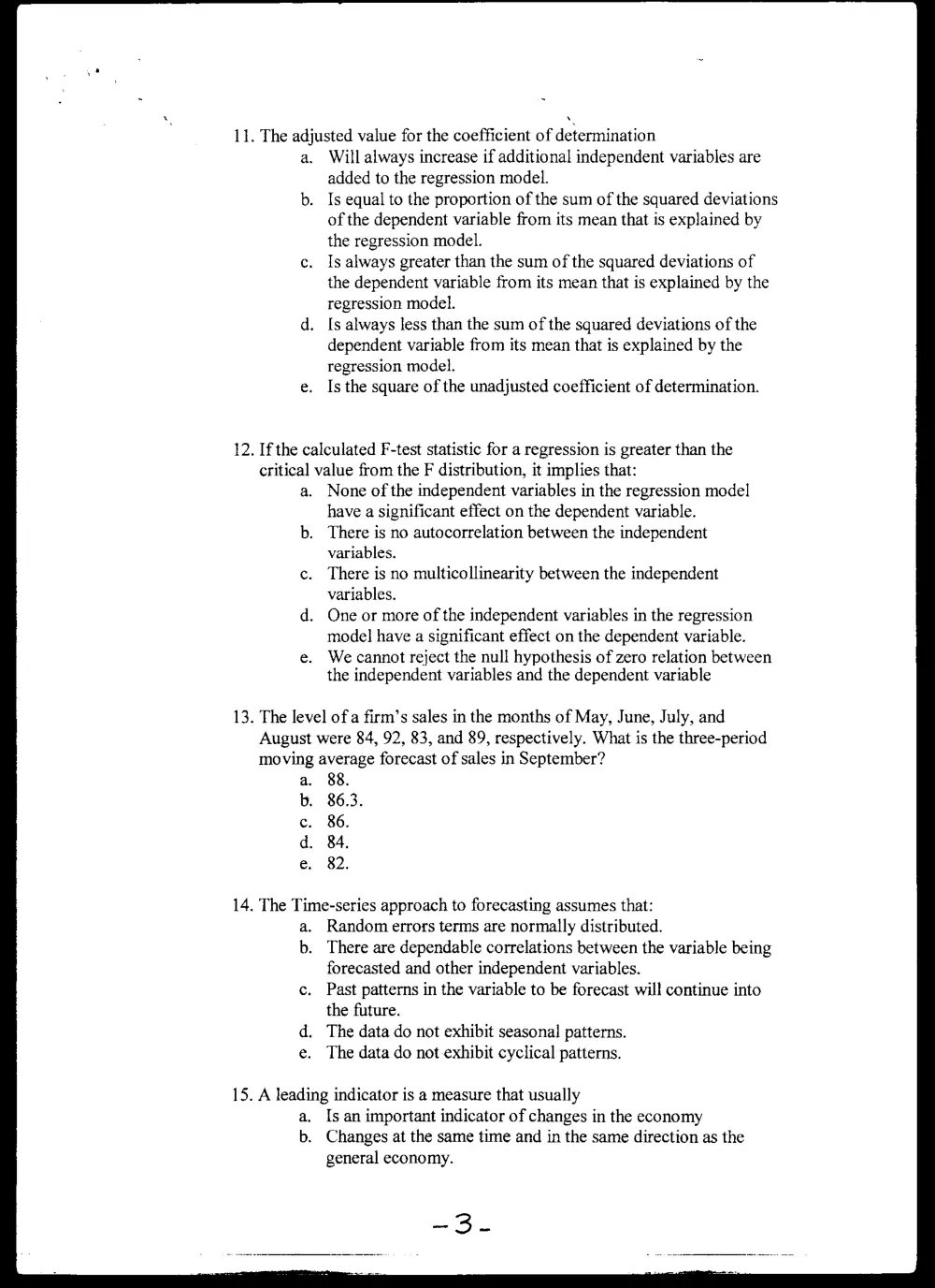
. ‘AMERICAN UNIVERSITY of BEIRUT SCHOOL of BUSINESS BUSS 230 MID-TERM EXAM - November 18, 2002 NAME: 1D: SECTION: INSTRUCTOR: ANSWER ALL QUESTIONS — TIME ALLOWED: 1 % hours L Multiple choice - (30 points). Circle the correct answer 1. The modern theory of the firm postulates that the primary objective of managers is to maximize: . The firm’s total revenue. . The value of the firm’s output. . The present value of the firm’s expected future profits. . The firm’s contribution to social welfare. . The wealth of the firm’s employees and customers. . Which of the following is the best definition of economic profit? . Business profit minus implicit costs. . Total revenue minus total explicit costs. . Total revenue minus total implicit costs. . Business profit minus explicit costs. . Explicit revenues minus implicit costs. . Ifthe price ofa good increases while the quantity of the good exchanged on markets increases also, then the most likely explanation is that there has been: . An increase in demand. . A decrease in demand. . An increase in supply. . A decrease in supply. . A decrease in demand accompanied by an increase in supply. . If marginal revenue is equal to zero, then: Total profit is zero also: b. Average revenue is zero also. c. Total revenue is at a maximum. d. Average revenue is at a maximum. e. Total cost is at a minimum. . The marginal principle asserts that, in general, when NET BENEFIT is maximized a. Total benefit will be equal to total cost. b. Average benefit will be equal to average cost. Cc. d. G. Marginal benefit will be equal to marginal cost. Average cost will be above average revenue but below average benefit. Total benefit will be at a maximum. 6. Ifboth average cost (AC) and marginal cost (MC) are U shaped, then a. b. c d. e. AC will reach a minimum at a level of output that is less than that at which MC reaches a minimum. The total cost curve will be a straight line. AC will reach a minimum at a level of output that is greater than that at which MC reaches a minimum. Both AC and MC will reach a minimum at the same level of output. AC will be always below MC. . Assuming a demand function of the form Q = 24 - 2P. AtP = 6, the price elasticity of demand is: There i is not enough information to arrive at an answer. _ As the economic recession worsened in 2001, household income fell by 5%. Over the same period, total expenditures on automobile repairs increased by 3%. Assuming no change in all other economic variables affecting houschold expenditures : The income elasticity of demand is equal to 0.6. . Automobile repairs must be a normal good. Automobile repairs must be an inferior good. . The price elasticity of demand for automobile repairs is equal to -5/3. The price elasticity of demand for automobile repairs is equal to -3 . Ifthe price of a good increases, then a. b. c. d. e. The demand for complementary goods will increase. The demand for the good will increase. The demand for substitute goods will decrease. The demand for the good will decrease. Total expenditures on the good will increase. -_—. 10. Application of simple linear regression analysis to the estimation ofa demand function yielded the following result: Q = 24 - 2P. Ifat the price P = 6, was Q = 10, then the crror (e) for that price/quantity observation is: Zero. ‘ 11. The adjusted value for the coefficient of determination a. Will always increase if additional independent variables are added to the regression model. b. Is equal to the proportion of the sum of the squared deviations of the dependent variable from its mean that is explained by the regression model. Is always greater than the sum of the squared deviations of the dependent variable from its mean that is explained by the regression model. . Is always less than the sum of the squared deviations of the dependent variable from its mean that is explained by the regression model. e. Is the square of the unadjusted coefficient of determination. 12. If the calculated F-test statistic for a regression is greater than the critical value from the F distribution, it implies that: a. None of the independent variables in the regression model have a significant effect on the dependent variable. b. There is no autocorrelation between the independent variables. There is no multicollinearity between the independent variables. One or more of the independent variables in the regression model have a significant effect on the dependent variable. We cannot reject the null hypothesis of zero relation between the independent variables and the dependent variable 13. The level of a firm’s sales in the months of May, June, July, and August were 84, 92, 83, and 89, respectively. What is the three-period moving average forecast of sales in September? 88. 86.3. 86. 84. 82. 14. The Time-series approach to forecasting assumes that: a. Random errors terms are normally distributed. b. There are dependable correlations between the variable being forecasted and other independent variables. c. Past patterns in the variable to be forecast will continue into the future. d. The data do not exhibit seasonal patterns. e. The data do not exhibit cyclical patterns. 15. A leading indicator is a measure that usually a. Is an important indicator of changes in the economy b. Changes at the same time and in the same direction as the general economy. Changes in the same direction as the general economy before the general economy changes. . Causes changes in the general economy. Indicates the performance of the leading industries of the economy. 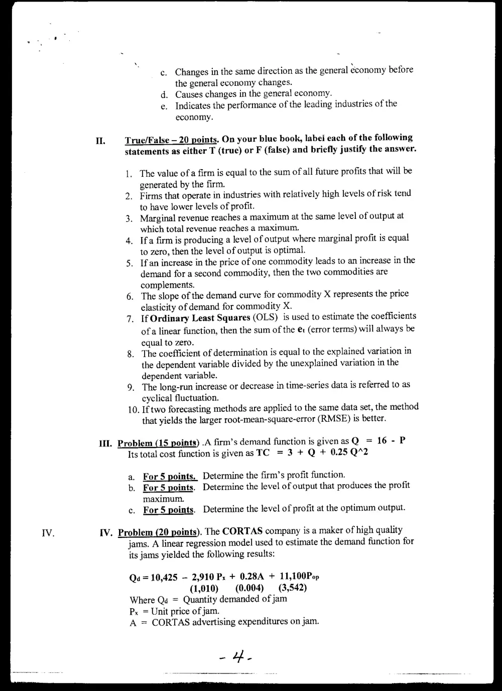True/False — 20 points. On your blue book, labei each of the following statements as either T (true) or F (false) and briefly justify the answer. L. 2. The value of a firm is equal to the sum of all future profits that will be generated by the firm. Firms that operate in industries with relatively high levels of risk tend to have lower levels of profit. . Marginal revenue reaches a maximum at the same level of output at which total revenue reaches a maximum. . Ifa firm is producing a level of output where marginal profit is equal to zero, then the level of output is optimal. _ [fan increase in the price of one commodity leads to an increase in the demand for a second commodity, then the two commodities are complements. . The slope of the demand curve for commodity X represents the price elasticity of demand for commodity X. . If Ordinary Least Squares (OLS) is used to estimate the coefficients ofa linear function, then the sum of the et (error terms) will always be equal to zero. _ The coefficient of determination is equal to the explained variation in 9. 10. the dependent variable divided by the unexplained variation in the dependent variable. The long-run increase or decrease in time-series data is referred to as cyclical fluctuation. If two forecasting methods are applied to the same data set, the method that yields the larger root-mean-square-error (RMSE) is better. Il. Problem (15 points) .A firm’s demand function is givenasQ = 16 - P Its total cost function is givenas TC = 3 + Q + 0.25 Q%2 a. b. c. For 5 points. Determine the firm’s profit function. For 5 points. Determine the level of output that produces the profit maximum. For 5 points. Determine the level of profit at the optimum output. IV. Problem (20 points). The CORTAS company is a maker of high quality jams. A linear regression model used to estimate the demand function for its jams yielded the following results: Qa = 10,425 — 2,910 Px + 0.28A + 11,100Pop (1,010) (0.004) (3,542) Where Qe = Quantity demanded of jam Px = Unit price of jam. A = CORTAS advertising expenditures on jam. 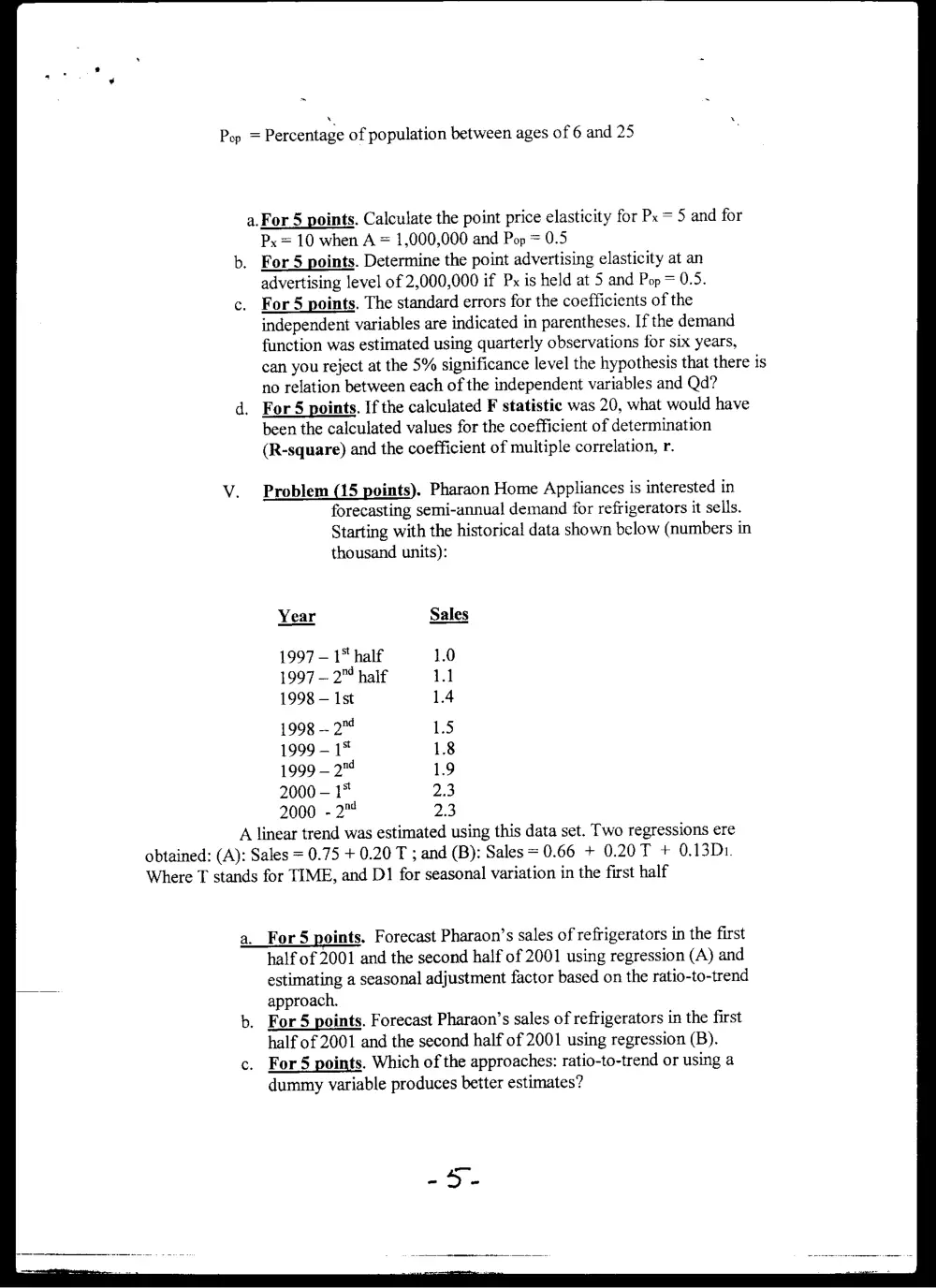_ Ye x Pop = Percentage of population between ages of 6 and 25 a.For 5 points. Calculate the point price elasticity for Px = 5 and for Px = 10 when A = 1,000,000 and Pop = 0.5 . For 5 points. Determine the point advertising elasticity at an advertising level of 2,000,000 if Px is held at 5 and Pop = 0.5. . For 5 points. The standard errors for the coefficients of the independent variables are indicated in parentheses. If the demand function was estimated using quarterly observations for six years, can you reject at the 5% significance level the hypothesis that there is no relation between each of the independent variables and Qd? . For 5 points. If the calculated F statistic was 20, what would have been the calculated values for the coefficient of determination (R-square) and the coefficient of multiple correlation, r. Problem (15 points). Pharaon Home Appliances is interested in forecasting semi-annual! demand for refrigerators it sells. Starting with the historical data shown below (numbers in thousand units): Year Sales 1997 — 1" half 1.0 1997 — 2™ half 1.1 1998 — Ist 1.4 1998 — 24 1.5 1999 - 1* 1.8 1999-2" 1.9 2000 — 1° 2.3 2000 - 2™ 2.3 A linear trend was estimated using this data set. Two regressions ere obtained: (A): Sales = 0.75 + 0.20 T ; and (B): Sales = 0.66 + 0.20 T + 0.13D1. Where T stands for TIME, and D1 for seasonal variation in the first half a._For 5 points, Forecast Pharaon’s sales of refrigerators in the first half of 2001 and the second half of 2001 using regression (A) and estimating a seasonal adjustment factor based on the ratio-to-trend approach. b. For 5 points. Forecast Pharaon’s sales of refrigerators in the first half of 2001 and the second half of 2001 using regression (B). c. For5 points. Which of the approaches: ratio-to-trend or using a dummy variable produces better estimates? 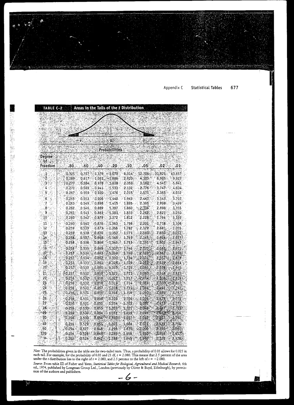Appendix C Statistical Tables 677 Note: The probabilities given in the table are for ewo-tailed tests. Thus, a probability of 0.05 allows for 0.025 in each tail. For example, for the probability of 0.05 and 21 df, t = 2.080. This means that 2.5 percent of the area under the ¢ distribution lies to the right of t = 2.080, and 2.5 percent to the left of t = —2.080. Source: From table II] of Fisher and Yates, Statistical Tables for Biological, Agricultural and Medical Research, 6th ed., 1974, published by Longman Group Ltd., London (previously by Oliver & Boyd, Edinburgh), by permis- sion of the authors and publishers. S Degrees of Freedom for Numerator 5 6 7 8 9 10 12 15 161 200 216 225 230 234 237 239 241 242 244 246 248 249 250 251 252 18.5 19.0 19.2 19.2 19.300 19.3 194 194 194 194 194 19.4 19.5 19.5 19.5 19.5 19.5 1.1 9.55 9.28 9.12 9.01 8.94 8.89 8.85 8.81 8.79 8.74 8.70 8.66 8.64 8.62 8.59 8.57 7.71 6.94 6.59 6.39 6.26 6.16 6.09 6.04 6.00 5.96 5.91 5.86 5.80 5.77 5.75 5.72 5.69 6.61 5.79 5.41 5.19 5.05 4.95 4.88 4.82 477 4.74 4.68 4.62 4.56 4.53 4.50 4.46 4.43 5.99 5.14 4.76 4.53 4.39 4,28 4.21 415 410 4.06 4.00 3.94 3.87, 3.84 3.81 3.77 3.74 5.59 4.74 435 422 3.97 3.87 3.79 3.73 3.68 = 3.64 3.57 3.51 3.44 3.44 3.38 3.34° 3.30 5.32 446 4.07 3.84 3.69 3.58 3.50 3.44 3.39 3.35 3.28 3.22 3.15 3.12 3.08 3.04, 3.01 5.12 4.26 3.86 3.63 3.48 3.37 3.29 3.230 3.18 93.14 3.07 3.01 2.94 2.90 2.86 2.83, 2.79 4.96 410 3.71 3.48 3.33 3.22 3.14 3.07 3.02 2.98 2.91 2.85 2.77 2.74 2.70 2.66! 2.62 4.84 3.98 3.59 3.36 3.20 3.09 3.01 2.95 2.90 2.85 2.79 2.72 2.65 2.61 2.57 2.53 2.49 4.75 3.89 3.49 3.26 3,11 3.00 2.91 2.85 2.80 2.75 2.69 2.62 2.54 2.51 2.47 2.43° 2.38 4.67 3.81 3.41 3.18 3.03 2.92 2.83 2.77 2.71 2.67 2.60 2.53 2.46 2.42 2,38. 2.34:. 2.30 4.60 3.74 3.34 ° 3.11 2.96 2.85 2.76 2.70 2.65 2.60 2.53 2.46 2.39 2:35 2.31 2.27. 2.22 4.54 3.68 — 3.29- . 3.06 2.90 2.79 271 2.64 259 2.54 2.48 2.40 2.33 > 2.29 2.25 2.20 2.16 449° 3,63 3.24 3.01 2.85 2.74 2.66 2.59 2.54 2.49 2.42 2.35 2.28 2.24 2.19 2.15 2.11 445 53,59 3.20. 2.96 2.81 2.70 2.61 2.55 2.48 2.45 2.38 2.31 2.23. 2.19 2.15° 2.10 | 2.06 A4L. 3.55°- 3,16 2.93 2.77 2.66 258 2.51 2.46 2.41 2.34 © 2.27 2.19. 2.15 2.11 2.06 © 2:02 4.38 3.52 3.13 2.90 2.74 2.63 2.54 248 2.42 2.39 2.31. 2.23 2.16: 2.41 2.07: 2.03. 1.98 4.35 3.49. 3,10 2.87 2.71 2.60 2.51 2.45 2.39 2.35 2.28 2.20 2.12. 2.08 2.04 1.99 1.95 4.32 ..3.47. 3.07...2.84 2.68 2.57 2.49 2.42 2.37 2,32 2.25 2.18 2.10° °2.05°°. 2.01 1:96°...4.92 4.30. 3144. 3.05. 2.82 2.66 2.55 246 240 2.34 2.30 2.23 2.15 2.07. 2,03... 1.98 1.94: ; 2:89 4.28 3.42. 3.03 2.80 2.64 2.53 2.44 2.37 2.32 2.27 2.20) 2.13 2,05 -.) 2:01 1.96 1.94. -2.86 4.26 3.40 - 3.02 2.78 . 2.62 2.51 2.42 236 2.30 2.25 2.18 2.41 2,03, --1.98 1.94 4.89 1.84 4.24 23,39. 2.99 2:76 2.60 2.49 2:40 2.34 2.28 2.24 - 2.16 2.09 2.01. 1.96 892.07 1.87. 182: 5 g % £ = ° 2 5 a 5 s —E c=] a. 3 8 e & ba °o a 3 Hy & o a 417° »3.32 2.92) 2.69 2,53 2.42 2.330 2.27) 2.21 2.16 2.09 2.02 1.93. 1.89 1:84. 1.79" “2.74 4.08 3.23 © 2.84 2.61 2.45 2.34 225 2.38 2.12 2.08 2.00 1.92 1.84 -1.79 1.74 1.69" 7.64 4.00° 3.15. 2.76 = 2.53 2.37 2.25 2.17 2.10 2.04 1.99 1.92 1.84 1.75°°-1.70 1.65 159° * 1:53. 3.92 3.07 2.68 - 2.45 2.29 2.18 2.09 2.02 1.96 1.91 1.83 1.75 1.66 1.61 1.55 1.50 -.-1.43. 3.84 3.00 2.60 2.37 2.21 2.10 2.01 1.94 1.88 1.83 1.75 1.67 1.57. 1.52 1.46. 1.39) 4.3255 1:22 M. Merrington and C. M. Thompson, “Tables of Percentage Points of the Inverted Beta (F) Distribution,” Biometrica, vol. 33, 1943, p. 73.