BUSS 230 Midterm, Spring 2005

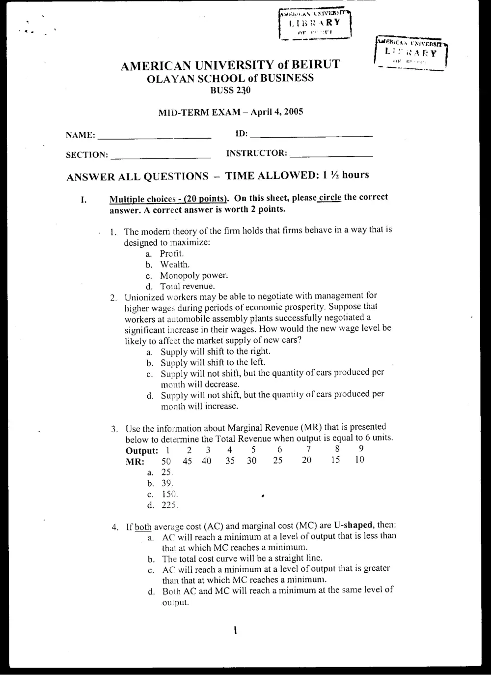
OT MrhtCAN UNIVERSIT LIBRARY ae . - hs en OL Ce] AMERICAN UNIVERSITY of BEIRUT [ a OLAYAN SCHOOL of BUSINESS BUSS 230 MID-TERM EXAM - April 4, 2005 NAME: ID: SECTION: INSTRUCTOR: ANSWER ALL QUESTIONS — TIME ALLOWED: | % hours I. Multiple choices - (20 points). On this sheet, please circle the correct answer. A correct answer is worth 2 points. 1. The modern theory of the firm holds that firms behave in a way that is designed to maximize: a. Profit. b. Wealth. c. Monopoly power. d. Total revenue. 2. Unionized workers may be able to negotiate with management for higher wages during periods of economic prosperity. Suppose that workers at automobile assembly plants successfully negotiated a significant increase in their wages. How would the new wage level be likely to affect the market supply of new cars? a. Supply will shift to the right. b. Supply will shift to the left. c. Supply will not shifi, but the quantity of cars produced per month will decrease. d. Supply will not shift, but the quantity of cars produced per month will increase. Use the information about Marginal Revenue (MR) that is presented below to determine the Total Revenue when output is equal to 6 units. Output: 1 2 3 4 5 6 7 8 9 MR: 50 45 40 35 30 25 20 15 10 a. 25. b. 39. c. 150. ’ d. 225. If both average cost (AC) and marginal cost (MC) are U-shaped, then: a. AC will reach a minimum at a level of output that is less than that at which MC reaches a minimum. b. The total cost curve will be a straight line. c. AC will reach a minimum at a level of output that is greater than that at which MC reaches a minimum. d. Both AC and MC will reach a minimum at the same level of output. 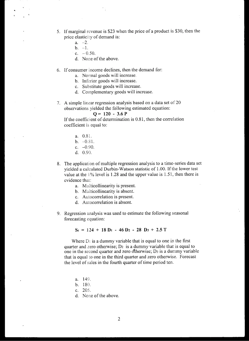If marginal revenue is $23 when the price of a product is $30, then the price elasticity of demand is: a. —2. b. -1. ec. —0.50. d. None of the above. If consumer income declines, then the demand for: a. Normal goods will increase. b. Inferior goods will increase. c. Substitute goods will increase. d. Complementary goods will increase. A simple linear regression analysis based on a data set of 20 observations yielded the following estimated equation: Q= 120 - 3.6P If the coefficient of determination is 0.81, then the correlation coefficient is equal to: a. 0.81. b. -0.81. c. -0.90. d. 0.90. The application of multiple regression analysis to a time-series data set yielded a calculated Durbin-Watson statistic of 1.00. If the lower test value at the 1% level is 1.28 and the upper value is 1.51, then there is evidence that: a. Multicollinearity is present. b. Multicollinearity is absent. c. Autocorrelation is present. d. Autocorrelation is absent. Regression analysis was used to estimate the following seasonal forecasting equation: St = 124 + 18Di - 46 D2 - 28 D3 + 2.5T Where D: is a dummy variable that is equal to one in the first quarter and zero otherwise; D2 is a dummy variable that is equal to one in the second quarter and zero otherwise; D3 is a dummy variable that is equal to one in the third quarter and zero otherwise. Forecast the level of sales in the fourth quarter of time period ten. a. 149, b. 180. c. 205. d. None of the above. 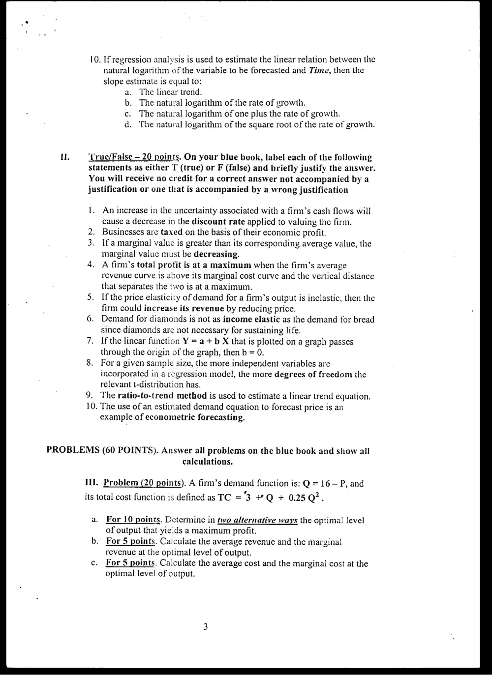10. If regression analysis is used to estimate the linear relation between the natural logarithm of the variable to be forecasted and Time, then the slope estimate is equal to: a. The linear trend. b. The natural logarithm of the rate of growth. c. The natural logarithm of one plus the rate of growth. d. The natural logarithm of the square root of the rate of growth. ‘Lrue/False — 20 points. On your blue beok, label each of the following statements as either T (true) or F (false) and briefly justify the answer. You will receive no credit for a correct answer not accompanied by a justification or one that is accompanied by a wrong justification 1. An increase in the uncertainty associated with a firm’s cash flows will cause a decrease in the discount rate applied to valuing the firm. Businesses are taxed on the basis of their economic profit. Ifa marginal value is greater than its corresponding average value, the marginal value must be decreasing. A firm’s total profit is at a maximum when the firm’s average revenue curve is above its marginal cost curve and the vertical distance that separates the two is at a maximum. If the price elasticity of demand for a firm’s output is inclastic, then the firm could increase its revenue by reducing price. Demand for diamonds is not as income elastic as the demand for bread since diamonds are not necessary for sustaining life. If the linear function Y = a + b X that is plotted on a graph passes through the origin of the graph, then b = 0. For a given sample size, the more independent variables are incorporated in a regression model, the more degrees of freedom the relevant t-distribution has. The ratio-to-trend method is used to estimate a linear trend equation. . The use of an estimated demand equation to forecast price is an example of econometric forecasting. PROBLEMS (60 POINTS). Answer all problems on the blue book and show all calculations. III. Problem (20 points). A firm’s demand function is: Q = 16 — P, and its total cost function is defined as TC = "3 ¥ Q + 0.25 Q?. a. For 10 points. Determine in hve alternative ways the optimal level of output that yields a maximum profit. b. For 5 points. Calculate the average revenue and the marginal revenue at the optimal level of output. For 5 points. Calculate the average cost and the marginal cost at the optimal level of output. 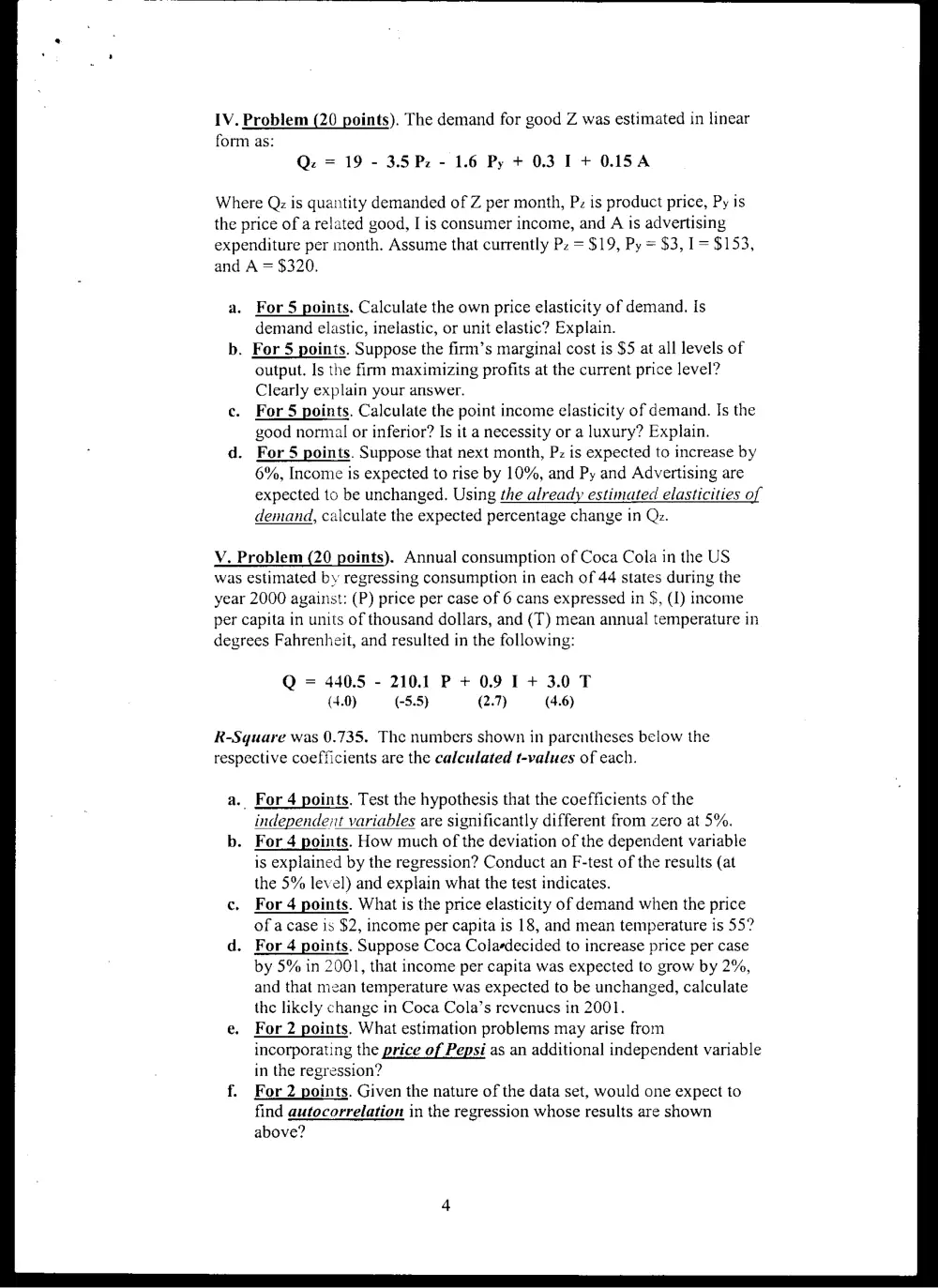IV. Problem (20 points). The demand for good Z was estimated in linear form as: Q. = 19 - 3.5 Pz - 1.6 Py + 0.3 1+ O.1SA Where Qz is quantity demanded of Z per month, Pz is product price, Py is the price of a related good, I is consumer income, and A is advertising expenditure per month. Assume that currently Pz = $19, Py = $3, 1= $153, and A = $320. a. For 5 points. Calculate the own price elasticity of demand. Is demand elastic, inelastic, or unit elastic? Explain. b. For 5 points. Suppose the firm’s marginal cost is $5 at all levels of output. Is the firm maximizing profits at the current price level? Clearly explain your answer. For 5 points. Calculate the point income elasticity of demand. Is the good normal or inferior? Is it a necessity or a luxury? Explain. . For 5 points. Suppose that next month, Pz is expected to increase by 6%, Income is expected to rise by 10%, and Py and Advertising are expected to be unchanged. Using the already estimated elasticities of demand, calculate the expected percentage change in Qz. V. Problem (20 points). Annual consumption of Coca Cola in the US was estimated by regressing consumption in each of 44 states during the year 2000 against: (P) price per case of 6 cans expressed in $, (1) income per capita in units of thousand dollars, and (T) mean annual temperature in degrees Fahrenheit, and resulted in the following: Q = 440.5 - 210.1 P + 0.9 I+ 3.0 T (4.0) (-5.5) (2.7) (4.6) R-Square was 0.735. The numbers shown in parentheses below the respective coefficients are the calculated t-values of each. .. For 4 points. Test the hypothesis that the coefficients of the independent variables are significantly different from zero at 5%. . For 4 points. How much of the deviation of the dependent variable is explained by the regression? Conduct an F-test of the results (at the 5% level) and explain what the test indicates. For 4 points. What is the price elasticity of demand when the price of a case is $2, income per capita is 18, and mean temperature is 55? . For 4 points. Suppose Coca Colaedecided to increase price per case by 5% in 2001, that income per capita was expected to grow by 2%, and that mean temperature was expected to be unchanged, calculate the likely change in Coca Cola’s revenues in 2001. For 2 points. What estimation problems may arise from incorporating the price of Pepsi as an additional independent variable in the regression? For 2 points. Given the nature of the data set, would one expect to find autocorrelation in the regression whose results are shown above? 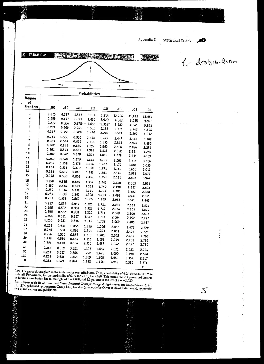Appendix C B TABLE C-2 o) Probabilities -80 -60 -40 : -10 205 -02 01 0.325 0.727 = 1.376 A 6.314 12.706 31.821 63.657 0.289 0.617 1,061 . 2.920 4.303 6.965 9.925 0.277 . 0.584. .0.978- --1. 2.353" 3.182 4.541 5.841 0.271 0.569 0.941 . 2.132 2.776 3.747 4.604 0.267 0.559 0,920 . 2.015 2.571 3.365 4.032 0.265 0.553 0.906 440 1,943 2.447 3.143 3.707 0.263 0.549 0.896 . 1.895 2.365 2.998 3.499 0.262 0.546 0.889 . 1.860 2.306 2.896 3.355 0.261 0,543 0,883 e 1.833 2.262 2.821 3.250 0.260 0.542 0,879 . 1.812 2.228 2.764 3.169 0.260 0.540 0.876 . 1.796 2.201 2.718 3.106 0.259 0.539 (0.873 : 1.782 2.179 2.681 3.055 0.259 0.538 0.870 . 1.771 2.160 2.650 * 3.012 0.258 0.537 0.868 “ 1.761 2.145 2.624 2.977 0.258 0.536 0.866 - 1.753 2.131 2.602 2.947 0.258 0.535 0.865 . 1.746 2.120 2.583 2.921 0.257 0.534 «0.863 - 1.740. 2.110 2.567 2.898 0.257 0.534 0,862 - 1.734 2.102 2.552 2.878 0.257 0.533 (0.861 . 1.729 2.093 2.539 2.861 0.257 0,533 0.860 . 1.725 2.086 2.528 2.845 0.257 0.532 0.859 . 1.721 2.080 2.518 2.831 0.256 0.532 0.858 . 1.717 2.074 2,508 2.819 0.256 0.532 0,858 . 1.714 2.069 2.500 2.807 0.256 0,531 0.857 . 1711 2.064 2.492 2,797 0.256 0.531 0.856 . 1.708 2.060 2.485 2.787 0.256 0.531 0.856 - 1.706 2.056 2.479 2.779 0.256 0.531 0,855 . 1.703 2,052 2.473 2.771 0.256 0.530 0.855 . 1.701 2,048 2.467 2.763 0.256 0.530 0.854 . 1.699 2.045 2.462 2.756 0,256 0.530 0.854 “ 1,697 2.042 2,457 2.750 0.255 0.529 0.851 . 1,684 2,021 2.423 2.704 0.254 0.527 0.848 - 1.671 2.000 2.390 2.660 0.254 0.526 0.845 . 1.658 1.980 2.358 2.617 0.253 0.524 0.842 . 1.645 1.960 2,326 2.576 r) + ~— Aste: The probabilities given in the table are for two-tailed tests. Thus, a probability of 0.05 allows for 0.025 in each mil. For example, for the probability of 0.05 and 21 df, t = 2.080. This means that 2.5 percent of the area wnder the ¢ distribution lies to the right of = 2,080, and 2.5 percent to the left of t = -2.080. 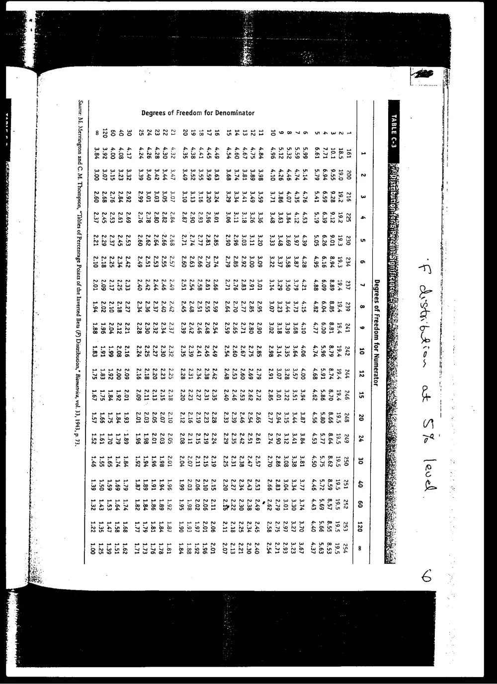Scarce: From table UI of Fi isher and Yates, Statistical Tables for Biological, Agricultural and Medical Research, 6th ed., 1974, published by Longman Group Ltd., London {previously by Oliver & Boyd, Edinburgh), by permis- sion of the authors and publishers, Statistical Tables t- TABLE C-3 Degrees of Freedom for Numerator 1 2 3 4 5 6 7 8 9 10 12 15 20 24 30 161 200 216 225 230 0-234 237 239 244 242 244 246 248 = 249 18.5 19.0 19.2 19.2 19.3 19.3 194 19.4 19.4 19.4 19.4 194 19.5 19.5 10.1 9,55 9.28 9.12 9.01 8.94 889 8.85 881 8.79 8.74 8.70 8.66 8.64 7.71 6.94 6.59 639 626 6.16 6.09 6.04 6.00 5.96 591 586 5.80 5.77 6.61 5.79 5.41 5.19 5.05 4.95 488 482 477 4.74 468 462 456 4.53 5.99 5:14 4.76 453 439 4.28 421 4.15 410 4,06 4.00 3.94 3.87 3.84 5.59 474 4.35 412 3.97 3.87 3.79 3.73 3.68 3.64 3.57 3.51 3.44 3.41 5.32 446 4.07 3.84 3.69 3.58 3.50 3.44 3.39 3.35 3.28 3.22 3.15 3.12 5.12 4.26 3.86 3.63 3.48 3,37 3.29 3.23 3.18 «03.14 3.07 3.01 2.94 = 2.90 4.96 4,10 3.71 3.48 3.33 3.22 3.144 3.07 3.02 2.98 2.91 2.85 2.77 2.74 4.84 3.98 3.59 3.36 3.20 3.09 3.01 2.95 290 2.85 2.79 2.72 2.65 2.61 4.75 3.89 3.49 3.26 3.11 3.00 2.91 2.85 280 2.75 2.69 2.62 2.54 2.51 4.67 3.81 3.41 3.18 3.03 2.92 2.83 2.77 2.71 2.67 2.60 2.53 2.46 2.42 4.60 3.74 3.34 3.11 2.96 2.85 2.76 2.70 2.65 2.60 2.53 246 2.39 2.35 4.54 3.68 3.29 3.06 2.90 2.79 2.71 2.64 2.59 2.54 2.48 2.40 2.33 2.29 449 3.639 3.24 3.01 2.85 2.74 2.66 2.59 254 2.49 2.42 2.35 2.28 2.24 445 3.59 3.20 2.96 2.81 2.70 2.61 2.55 248 2.45 2.38 2.31 2.23 2.19 4.41 3.55 3.16 2.93 2.77 2.66 2.58 2.51 246 2.41 2.34 2.27 2.19 2.15 4.38 3.52 3.13 2.90 2.76 2.63 2.54 2.48 242 2.39 2.31 2.23 2.16 2141 4.35 3.49 3.10 2.87 2.71 2.60 2.51 245 2.39 2.35 2.28 2.20 2.12 2.08 4.32 3.47 3.07 2.84 2.68 2.57 249° 2.42 2.37 2.32 2.25 2.18 2.10 2.05 4.30 3.44 3.05 2.82 2.66 2.55 2.46 2.40 2.34 2.30 2.23 2.15 2.07 2.03 4.28 3.42 3.03 2.80 2.64 2.53 244 2.37 232 2.27. 2.20 2.13 2.05 2.01 4.26 3.40 3.01 2.78 2.62 2.51 2.42 2.36 230 2.25 2.18 211. 2.03 1.98 4.24 3.39 2.99 2.76 260° 2.49 2.40 2.36 2.28 2.24 2.16 2.09 2.01 1.96 4.17 3.32 2.92 2.69 2.53 2.42 2.33 2.27 2.21 2.16 2.09 2.01 1.93 -1.89 4.08 3.23 286 2.61 245 2.346 2.25 218 212 208 2.00 1.92 184 1,79 4.00 3.15 2.76 2.53 2.37 2.25 2.17) 2.10 204 199 1.92 184 1.75 1,70 3,92 3.07 2.68 2.45 2.29 2.18 2.09 202 196 191 183 175 166 1.61 3.84 3.00 260 2.37 221 210 2.01 196 188 183 1.75 1.67 1.57 1.52 5 5 = £ E 5 i=} v a _ & E i=} a=] 3 3 2 = ha 5 a 8 3 a $ a Source: M. Merrington and C. M. Thompson, “Tables of Percentage Points of the Inverted Beta (F) Distribution,” Biometrica, vol. 33, 1943, p. 73.