BUSS 230 Midterm, Fall 2006

6 Reading Howes DSR FN) AMERICAN UNIVERSITY of BEIRUT OLAYAN SCHOOL of BUSINESS BUSS 230 MID-TERM EXAM - November 14, 2005 ID: NAME: SECTION: INSTRUCTOR: ANSWER ALL QUESTIONS — TIME ALLOWED: 1 1/2 hours Multiple choice questions - (24 points). On this sheet, please circle your answer. A correct answer is worth 2 points. 1. Monica quit her $40,000 a year job, purchased a warehouse that used to be rented out for $1,500 a month, and used the space to breed and sell tropical fish. In her first year she made a business profit of $60,000. What was her economic profit? a. $60,000. b. $42,000. c. $20,000. d. $2,000. 2. The tendency for managers to operate in a manner that maximizes their personal utility instead of firm profits is referred to as: . Consumer utility incentive. . Principal-agent problem. . Principal utility hypothesis. . Private benefit maximization. 3. The marginal principle asserts that, in general, when net benefit is maximized: a. Total benefit will be equal to total cost. b. Average benefit will be equal to average cost. c. Marginal benefit will be equal to marginal cost. d. Average cost will be above total cost but below average benefit. 4. If an average curve has a negative slope, then the corresponding: a. Marginal curve is below the average curve. b. Total curve has a negative slope. c. Marginal curve is above the average curve. d. Total curve has a positive slope. 10. 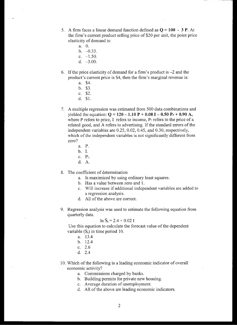A firm faces a linear demand function defined as Q= 100 - 3 P. At the firm’s current product selling price of $20 per unit, the point price elasticity of demand is: a. 0. b. ~0.33. ec. —1.50. d. —3.00. If the price elasticity of demand for a firm’s product is -2 and the product’s current price is $4, then the firm’s marginal revenue is: a. $4. b. $3. ec. $2. d. $1. A multiple regression was estimated from 500 data combinations and yielded the equation: Q = 120 - 1.10 P + 0.08 I - 0.50 Pr + 0.90 A, where P refers to price, I refers to income, Pr refers to the price of a related good, and A refers to advertising. If the standard errors of the independent variables are 0.25, 0.02, 0.45, and 0.30, respectively, which of the independent variables is not significantly different from zero? a. P. b. I. c. Pr. d. A. The coefficient of determination a. Is maximized by using ordinary least squares. b. Has a value between zero and 1. c. Will increase if additional independent variables are added to a regression analysis. d. All of the above are correct. Regression analysis was used to estimate the following equation from quarterly data. In S,= 2.4 + 0.02 t Use this equation to calculate the forecast value of the dependent variable (S,) in time period 10. a. 13.4 b. 12.4 c. 2.6 d. 2.4 Which of the following is a leading economic indicator of overall economic activity? ; Commissions charged by banks. Building permits for private new housing. Average duration of unemployment. All of the above are leading economic indicators. 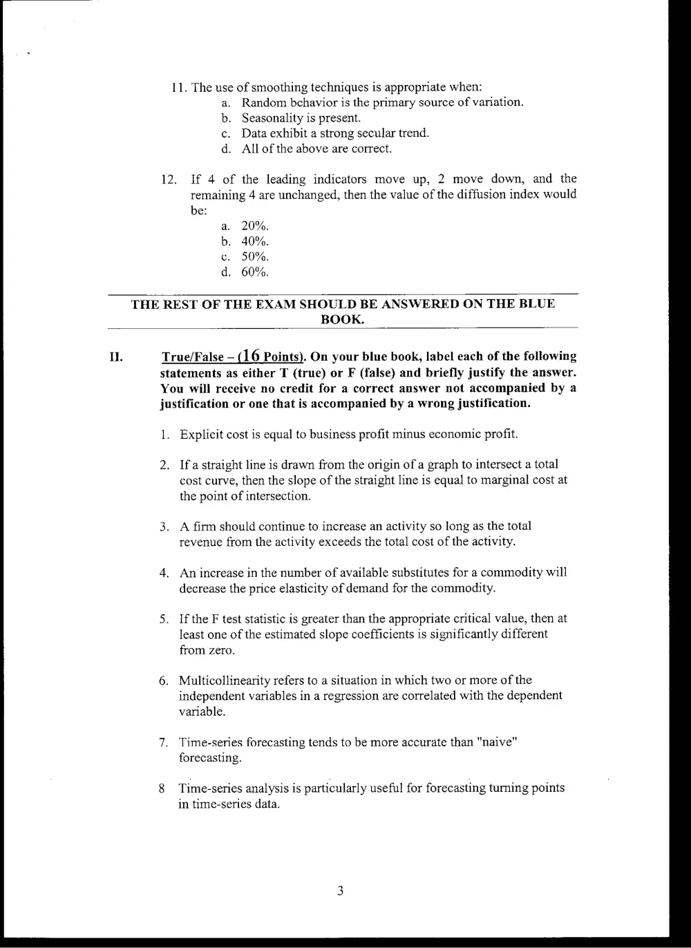ao Fp 2 11. The use of smoothing techniques is appropriate when: a. Random behavior is the primary source of variation. Seasonality is present. Data exhibit a strong secular trend. All of the above are correct. If 4 of the leading indicators move up, 2 move down, and the remaining 4 are unchanged, then the value of the diffusion index would be: 20%. 40%. 50%. 60%. THE REST OF THE EXAM SHOULD BE ANSWERED ON THE BLUE BOOK. True/False — (16 Points). On your blue book, label each of the following statements as either T (true) or F (false) and briefly justify the answer. You will receive no credit for a correct answer not accompanied by a justification or one that is accompanied by a wrong justification. 1. 2. Explicit cost is equal to business profit minus economic profit. If a straight line is drawn from the origin of a graph to intersect a total cost curve, then the slope of the straight line is equal to marginal cost at the point of intersection. A firm should continue to increase an activity so long as the total revenue from the activity exceeds the total cost of the activity. An increase in the number of available substitutes for a commodity will decrease the price elasticity of demand for the commodity. If the F test statistic is greater than the appropriate critical value, then at least one of the estimated slope coefficients is significantly different from zero. Multicollinearity refers to a situation in which two or more of the independent variables in a regression are correlated with the dependent variable. Time-series forecasting tends to be more accurate than "naive" forecasting. Time-series analysis is particularly useful for forecasting turning points in time-series data. 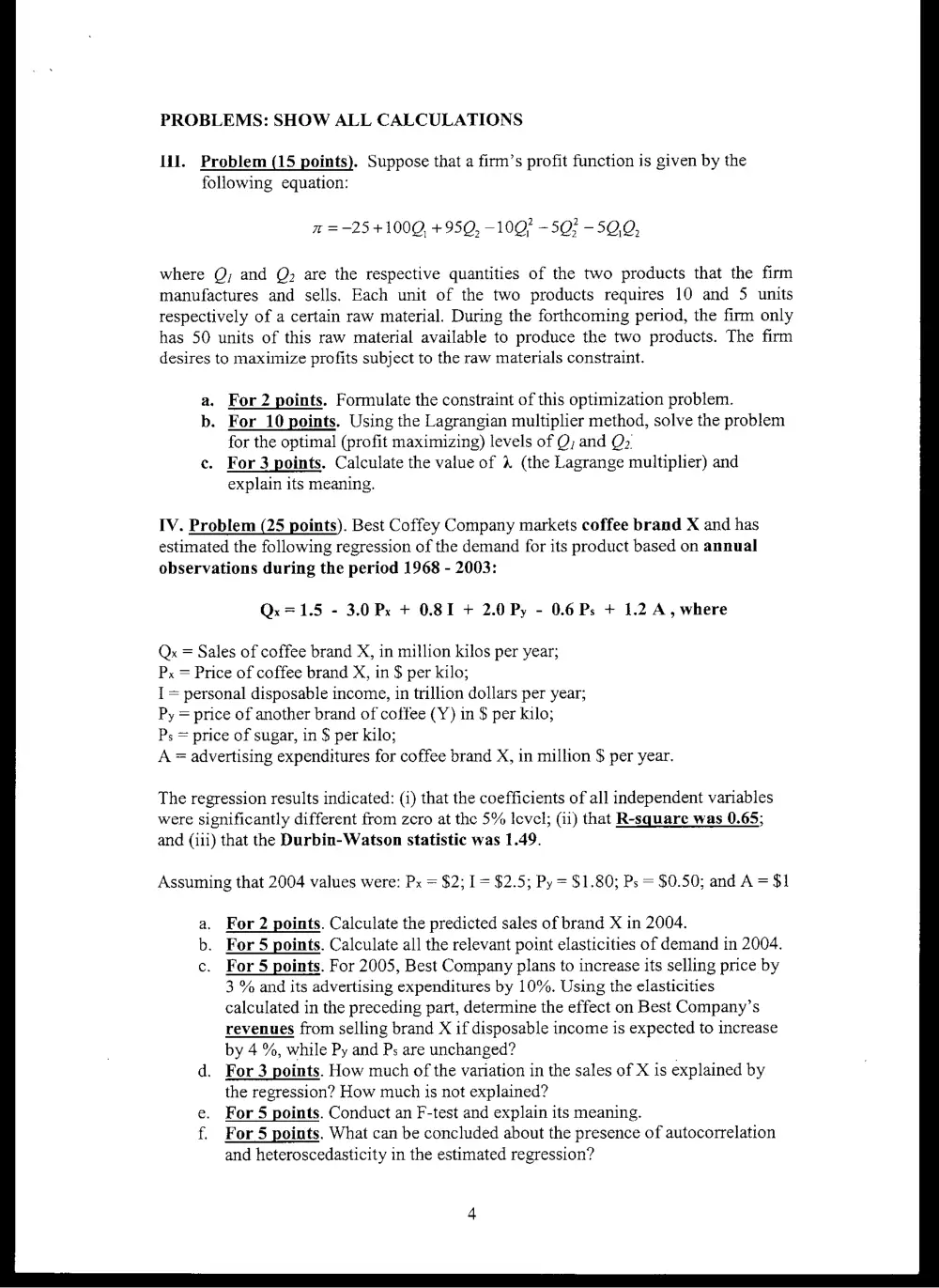PROBLEMS: SHOW ALL CALCULATIONS Il. Problem (15 points). Suppose that a firm’s profit function is given by the following equation: m =-25 +1000, +950, -100? -50? -5Q,0, where Q; and Q are the respective quantities of the two products that the firm manufactures and sells. Each unit of the two products requires 10 and 5 units respectively of a certain raw material. During the forthcoming period, the firm only has 50 units of this raw material available to produce the two products. The firm desires to maximize profits subject to the raw materials constraint. a. For 2 points. Formulate the constraint of this optimization problem. b. For 10 points. Using the Lagrangian multiplier method, solve the problem for the optimal (profit maximizing) levels of Q; and Qy c. For 3 points, Calculate the value of 4 (the Lagrange multiplier) and explain its meaning. IV. Problem (25 points). Best Coffey Company markets coffee brand X and has estimated the following regression of the demand for its product based on annual observations during the period 1968 - 2003: Qx=1.5 - 3.0 Px + 0.81 + 2.0 Py - 0.6 Ps + 1.2 A, where Qx = Sales of coffee brand X, in million kilos per year; Px = Price of coffee brand X, in $ per kilo; I= personal disposable income, in trillion dollars per year; Py = price of another brand of coffee (Y) in $ per kilo; Ps = price of sugar, in $ per kilo; A = advertising expenditures for coffee brand X, in million $ per year. The regression results indicated: (i) that the coefficients of all independent variables were significantly different from zero at the 5% level; (ii) that R-square was 0.65; and (iii) that the Durbin-Watson statistic was 1.49. Assuming that 2004 values were: Px = $2; 1 = $2.5; Py = $1.80; Ps = $0.50; and A= $1 a. For 2 points. Calculate the predicted sales of brand X in 2004. b. For 5 points. Calculate all the relevant point elasticities of demand in 2004. c. For 5 points. For 2005, Best Company plans to increase its selling price by 3 % and its advertising expenditures by 10%. Using the elasticities calculated in the preceding part, determine the effect on Best Company’s revenues from selling brand X if disposable income is expected to increase by 4 %, while Py and Ps are unchanged? d. For 3 points. How much of the variation in the sales of X is explained by the regression? How much is not explained? For 5 points. Conduct an F-test and explain its meaning. f. For 5 points. What can be concluded about the presence of autocorrelation and heteroscedasticity in the estimated regression? o V. Problem (20 points). An ice-cream company’s sales exhibit a seasonal pattern, with higher sales during the spring and summer quarters and lower sales during the fall and winter quarters. The company developed the following sales forecasting model using data from the first quarter of 1990 to the last quarter of 2004: Y¥: =5.9 + 0.14 T- 1.09 Dit+ 3.39 Da+ 4.44 Dat Where: Yt = predicted sales in quarter t ($ million); T is a time trend; and Dit, Dat, and Dst are dummy variables for quarter 1 (winter), quarter 2 (spring), and quarter 3 (summer), respectively. The definition of the dummy variables is: Di: takes a value of 1 in the first quarter of each year and 0 in the other quarters; Da takes a value of 1 in the second quarter of each year and 0 in the other quarters; and D3: takes a value of 1 in the third quarter of each year and 0 in the other quarters. (a) (i) For 3 points. Based on the time (secular) trend, what conclusion can you draw regarding the change in ice-cream sales over time? (ii) For 5 points. Forecast sales of ice-cream during the winter quarter of 2006. (iii) For 5 points. Clearly explain why a dummy variable for quarter 4 (Fall quarter) was not included in the model. (b) For 7 points. The table below shows semi-annual demand (in 1,000s) for holidays. A simple linear trend was estimated using this data set and resulted in an intercept of 0.79 and a slope of 0.19. Period Amount Demanded 1995.1 1.0 1995.2 1.1 1996.1 1.4 1996.2 1.5 1997.1 1.8 1997.2 1.9 1998.1 2.3 1998.2 2.3 Use the ratio-to-trend method to calculate the seasonal adjustment factor for the second half of the year and then forecast the quantity demanded for 2000.2. te} Probabilities 80 -60 40 -20 -10 -05 02 -O1 MIR 1.727 41.276 3.070 G.oa4 z.TUD 31,827 63.657 0.289 0.617 «1.061 1.886 «2.920 4.303 6.965 9,925 » 0.27 Trin D684. 0:978+——4:638 25353 3.182 ~ 4.541 5.841 0.271 (0.569 0.941 1.533 2,132 2.776 3.747 4,604 9.267 0.559 0.920 1.476 2.015 2.571 3.365 4.032 0.265 0.553 0.906 1.440 1.943 2.447 3.143 3,707 0.263 0.549 0.896 1.415 1.895. 2,365 2.998 3.499 0.262 0.546 0.889 1.397 1.860 2.306 2.896 3.355 0.261 0.543 0.883 1.383 - 1.833 2.262 2.821 3.250 0.260 0.542 0.879 1.372 4.812 2.228 2.764 3.169 0.260 0.540 0.876 1.363 1.796 2,201 2.718 3.106 0.259 0.539 0.873 1.356 1.782 2.179 2.681 3.055 0.259 0.538 «0.870 «2.350 1.771 2.160 2.650 ° 3.012 0.258° 0.537 0.868 [2.345 1,761 2.145 2.624 2.977 0.258; 0.536. 0.866 » 2.341 1.753 2.131 2.602 2.947 0.258 «0.535 0.865 4.337 1.746 2,120 2,583 2,921 0.257 0,534 0.863 1.333 1.740 2110 «2.567, 2.898 0.257 0.534 0.862 1.330". 1.734 2101-25822 878 0.257 0,533 0,861 1.328 «1.729 2.093 2.539 2.861 0.257 0.533 0.860 1.325 - 1,725 2,086 ~— 2.528 2 845 0.257 0.532 0.859 «1.323 «1.721 2.080 2.518 2.831 0.256 0.532 -0.858 1.321 1.717. 2.074 2.508 2.819 0.256 0.532 0.858. 1.319 1.714 2.069 2.500 2.807 0.256 0.531 0.857 1.318 27211 2.064 2.492 2.797 0.256 0,531 0,856 . 1.316 1.708 2.060 2.485 2.787 0.256 0.531 0.856 1.335 1.706 2.056 2.479 2.779 0.256 0.531 0.855 1.314 1.703 2,052 2.473 2.771 0.256 0.530 0.855 1.313 ~ 1.701 2.048 2.467 2.763 0.256 0.530 0.854 1.311 1.699 2.045 2.462 2.756 0.256 0.530 0.854 1.310 1.697 2.042 2.457 2.750 0.255 0.529 0.851 _ 1,303 1.684 2.021 2.423 2.704 0.254 0.527 0.848 1.296 4.671 2.000 2.390 2.660 0.254 0.526 0.845 1.289 1.658 1,980 2.358 2.617 0.253. 0.524 0.842 1.282 1,645 1.960 2.326 2.576 eae oe Nore: The probabilities given in the table are for two-tailed tests. Thus, a probability of 0.05 allows for 0.025 in ech tail. For example, for the probability of 0.05 and 21 df, ¢ = 2.080, This means that 2.5 percent of the area under the t distribution lies to the right of t = 2,080, and 2.5 percent to the left of t = —2.080. Sswree: From table Hi of Fisher and Yates, Statistical Tables for Biological, Agricultural and Medical Research, 6th ed. 1974, published by Longman Group Ltd., London {previously by Oliver & Boyd, Edinburgh), by permis- sica of the authors and publishers. 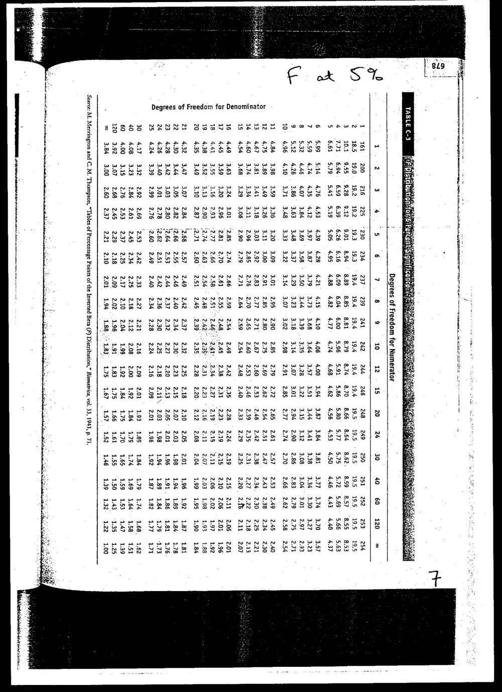TABLE C-3 Degrees of Freedom for Numerator 1. Pn 6 7 8 8 10 42. 15 20 161 216 = 225 234 237 239 241 242 244 246 248 249 250 251 18.5 19.2 19.2 19.3 19.4 19.4 19.4 19.4 194 194 19.5 19.5 | 19.5 19.5 10.1 9.28 9.12 8.94 8.89 8.85 881 879 8.74 8.70 866 864 8.62. 8.59 771 6.59 6.39 6.16 6.09 604 6.00 596 5.91 5.86 5.80 5.77 5.75 5.72 6.61 5.41 5,19 4.95 4.88 4.82 477° 474 468 462 456 453 450 4.46 5.99 : 4.76 4.53 4.28 4.21 4.15 4.10 406 4.00 3.94 3.87 3.84 3.81 3.77 5.59 435 4.12 3.87 3.79 3.73 3.68 3.64 3.57) 3.51 3.44 3.41 3,38 3.34 5.32 4.07 3.84 3.58 ~ 3.50 3.44 3.39 ..3.35 3.28 3.22 3.15 3.12 3.08 3.04 §.12 3,86 3.63 3.37 3.29 3.23 3.18 «03.44 «3.07 3.01 2.94 2.90 2.86 2.83 4.96 3,71 3.48 3.22 3.14 3.07 3.02 2.98 2.91 2.85 2.77 2.74 2.70 2.66 4.84 3.59 3.36 3.09 3.01 2.95 2.90 2.85 2.79 2.72 2.65 2.61 2,57 2.53 4,75 3.49 3.26 3.00 2.91 2.85 2.80 2.75 2.69 2.62 254 2.51 2.47 2,43 4.67 341 3.18 2.92 2.83 2.77 2.71 2.67 2.60 2.53 -2.46 2.42 2.38 2.34. 4.60 3.34 3.11 2.85 2.76 2.70 2.65 2.60 2.53 2.46 2.39 2.35 2.31 2.27 4.54 3.29 3.06 2.79 2.71 2.64 2.59 2.54 248 240 2.33 2.29 2.25 2.20 4.49 3.24 3.01 | 276 2.66 2.59 254 2.49 2.35 228 224 249 215 4.45 3.20 2.96 ° 2.70 2.61 2.55. 2.48. ..2.45 2.31 2.23: 2.19 2.15 2,20 4.41 3.16 2.93 - 2.66 2.58 2.515 2.46. 2.410 2 2.27° 249° 2.15 [211 © 2.06 4,38 3.13 2.90 2.63. 2.54 2.48 . 2.427 2:38: 2.23 ° 2.16 2.41 2.07 2.03 4.35 3.10 2.87 j 2.60°° 2.51 2.45 .2,39° 2.38 2.20, 2.12 2.08 2.04 . 1.99 4,32 3.07 2,84 257 249 2.42 2.37 2.32 2.18 2.10 2.05 2.01 1.96 4.30 3.05 2.82 2.55. 246 2.40 2.34 2.30 2.15 2.07 2.03, 198 1.94 4.28 3.03 2.80 ; 2.53 2.44 2.37 2.32 2.27 2.13 2.05 2.01 1.96 1.91, 4.26 3.01 2.78 42.62" 2.51 2.42 2.36 2.30 2.25 241 2.03 1.98 1.94. 1.89 4.24 2.99 2.76 :2.60° 249 2.40 2.34 2.28 2:24 2.09 2.01 196 192 1.87 4.17 2.92 2.69 (2.53 2.42 2.33 2.27 2.21. 2.16 2.01 193 1.89 1.84 1.79 4.08 2.84 2.61 2.45 2.34 2.25 2,18 2.12 2.08 1.92 184 1.79 1.74 1.69 4.00 2.76 2.53 2.37 2.25 2.17 2.10 2.04 = 1.99 1.84 4175 1.70 1.65 1.59 3.92 2.68 2.45 2.29 2.18 2.09 2.02 196 § 1.91 1750 (1.66 1.61 1.55 1.50 3.84 2.60 2.37 2.21 2.10 2:01, 1.94 1.88.,°: 1,83 167 157 152 © 1.46 1.39 OANA VaAWN o Coo Sk 2 o Pee ee aawn a ere aUA nN a nn ne yn Rw - o 2 oO =i —E o oc uv a = 2 § S 19 wv 2 uw % ° ” a 2 i=) uv a no w Aw ooo Source: M. Merrington and C. M. Thompson, “Tables of Percentage Points of the Inverted Bera (F) Distribution,” Biometrica, vol. 33, 1943, p. 73. ~ $0 1.50 4.59 1.46 1.63 1.42 1.67 1.38 1.72 1.34 77 55 1.83 1.60 1.49 4.64 1.45 1.68 1.41 1,72 1.38 1.77 60 1.55 1.62 1.51 1.65 1.48 1.69 1.44 1.73 1.41 1.77 Statistical Tables 613 Appendix C Durbin-Watson Statistic for 5 percent Significance Points of d, and dy & TABLE C-4 m4 Kn 2 Ka3 K=4 Kas - “a ay dy dy dy a dy a dy a, dy 15 1.08 1.36 0.95 4.54 0.82 V75 0.69 1.97 0.56 2:21 16 1.10 1.37 0.98 1.54 0.86 1.73 0.74 1.93 0.62 215 7 1.13 1.38 1.02 1.84 0.90 1.71 0.78 1.90 0.67 2.10 18 1.16 1.39 1.05 1.53 0.93 1.69 0.82 1.87 0.71 2.06 1 118 1.40 1.08 4.53 0.97 1.68 0.86 1.85 0.75 2.02 20 1.20 1.41 1.10 1.54 1.00 1.68 0.90 1.83 0.79 41.99 21 1.22 4.42 4.1300. 1.54 1.03 1.67 0.93 1.81 0.83 1.96 22 1.24 1.43 11S 1.54 1.05 1.66 0.96 1.80 0.86 1.94 23 1.26 1.44 V7 1.54 1.08 1.66 0.99 1.79 0,90 1.92 24 1.27 1.45 1.19 1.85 . 1.10 1.66 4.01 1.78 0.93 1,90 25 1.29 1.45 1.21 4,55 112 1.66 1.04. 1.77, 0.95 1.89 26 1.30 1.46 1.22 1.55 1.14 1.65 1.06 1.76 0.98 1.88 27 132°. 1.47 1.24 156 1.16 1.65 1.08 1.76 4.01 1.86 28 133° (1.48 126 1.56 1.18 1.65 1.10 1751.03 1.85 29 134 1.48 1271.56 1.20 1.65 112 174 1.05 1.84 30 1.35 1.49 1.28 1.57 1,21 1.65 1.14 1.74 1.07 1.83 KzI 1.36 4.50 4.30 1.57 1.23 1.65 1.16 1.74 1.09 1.83 32 1.37 1.50 1431 1.57 1.24 1.65 1.18 1.73 111 1.82 33 1.38 4.51 1.327 1.58 1.26 1.65 1.19 1.73 VA3 1.81 34 1.39 1.51 4.33 158 1,27 1.65 1.21 1.730 115 1.81 35 1.40 4.52 1.34 1.58 1.28 1.65 1.22 1.73 1.16 1.80 36 4.41 1.52 1.35 1.59 1,29 1.65 1.24 1.73 1.18 1.80 37 1.42 1.53 1.36 1.59 4.31 1.66 1.25 1.72 119 1.80 38 1.43 4.54 1.37 1.59 1.32 1.66 1.26 1.72 1.21 4.79 39 1.43 1.54 1.38 1.60 1.33 1.66 1.27 4.72 1,22 1.79 “40 1.44 1.54 1.39 1.60 1.34 1.66 1.29 1.72 1.23 1.79 45 4.48 1.57 1.43 1.62 1.38 1.67 1.34 1.72 1.29 1.78 6S 1.57 1.63 1.54 1.66 1.50 1.70 1.47, 1.73 1.44 1.77 70 1.58 1.64 155 1.67 1.52 1.70 1.49 1.74 1.46 75 1.60 1.65 1.57 1.68 1.54 1.71 1.S1 1.74 1.49 80 1.61 1.66 1.89 1.69 1.56 1.72 1.53 1.74 1.51 1.77 85 1.62 1.67 1.60 1.70 1.57 1.72 1.55 1.78 1.52 90 1.63 1,68 1.61 1,70 1,59 1.73 1.87 4.75 1.54 95 1.64 1.69 4.62 71 1.60 1.73 1.58 1.75 1.56 100 1.65 1.69 1.63 1.72 4.61 4.74 4.59 1.76 1.57 Note: n= number of observations; k’ = number of independent variables, Source: }. Durbin and G. $. Watson, “Testing for Serial Correlation in Least Squares Regression,” Biometrica, vol. 38, 1951, pp. 159-177. Reprinted with the permission of the authors and the trustees of Biometrica.