BUSS 230 Midterm, Fall 2013

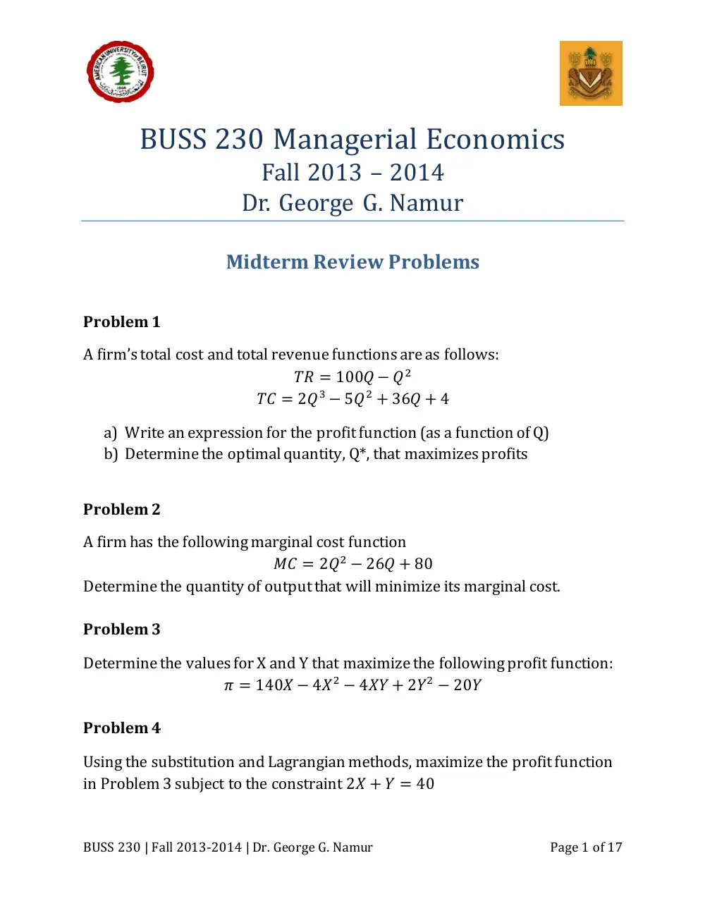
BUSS 230 | Fall 2013-2014 | Dr. George G. Namur Page 1 of 17 BUSS 230 Managerial Economics Fall 2013 – 2014 Dr. George G. Namur Midterm Review Problems Problem 1 A firm’s total cost and total revenue functions are as follows: a) Write an expression for the profit function (as a function of Q) b) Determine the optimal quantity, Q*, that maximizes profits Problem 2 A firm has the following marginal cost function Determine the quantity of output that will minimize its marginal cost. Problem 3 Determine the values for X and Y that maximize the following profit function: Problem 4 Using the substitution and Lagrangian methods, maximize the profit function in Problem 3 subject to the constraint BUSS 230 | Fall 2013-2014 | Dr. George G. 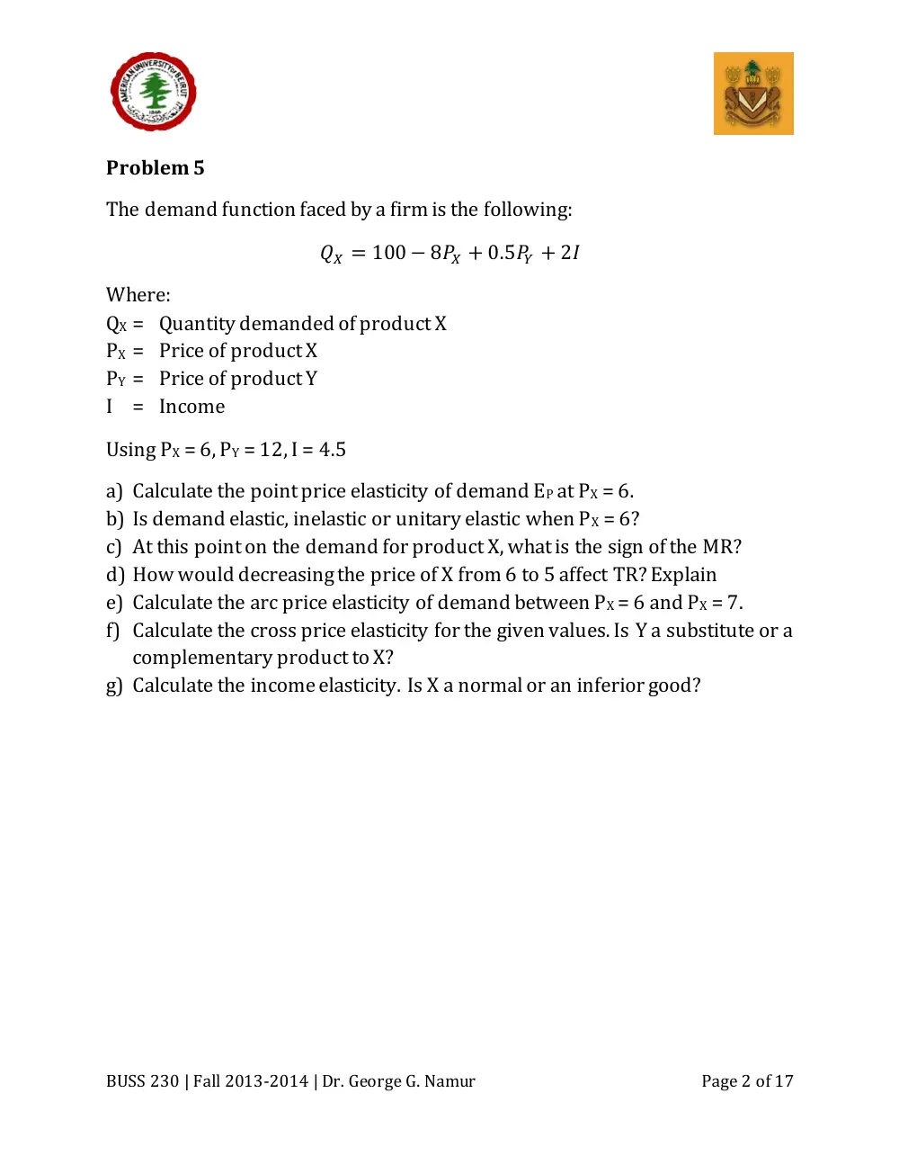Namur Page 2 of 17 Problem 5 The demand function faced by a firm is the following: Where: QX = Quantity demanded of product X PX = Price of product X PY = Price of product Y I = Income Using PX = 6, PY = 12, I = 4.5 a) Calculate the point price elasticity of demand EP at PX = 6. b) Is demand elastic, inelastic or unitary elastic when PX = 6? c) At this point on the demand for product X, what is the sign of the MR? d) How would decreasing the price of X from 6 to 5 affect TR? Explain e) Calculate the arc price elasticity of demand between PX = 6 and PX = 7. f) Calculate the cross price elasticity for the given values. Is Y a substitute or a complementary product to X? g) Calculate the income elasticity. Is X a normal or an inferior good? BUSS 230 | Fall 2013-2014 | Dr. George G. 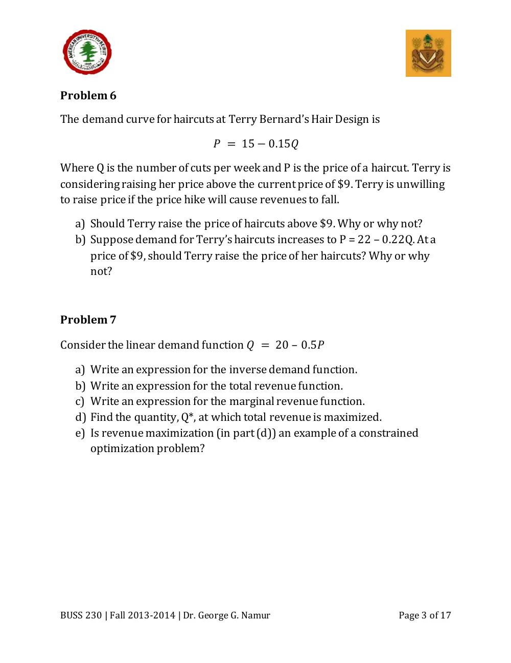Namur Page 3 of 17 Problem 6 The demand curve for haircuts at Terry Bernard’s Hair Design is Where Q is the number of cuts per week and P is the price of a haircut. Terry is considering raising her price above the current price of $9. Terry is unwilling to raise price if the price hike will cause revenues to fall. a) Should Terry raise the price of haircuts above $9. Why or why not? b) Suppose demand for Terry’s haircuts increases to P = 22 – 0.22Q. At a price of $9, should Terry raise the price of her haircuts? Why or why not? Problem 7 Consider the linear demand function – a) Write an expression for the inverse demand function. b) Write an expression for the total revenue function. c) Write an expression for the marginal revenue function. d) Find the quantity, Q*, at which total revenue is maximized. e) Is revenue maximization (in part (d)) an example of a constrained optimization problem? BUSS 230 | Fall 2013-2014 | Dr. George G. 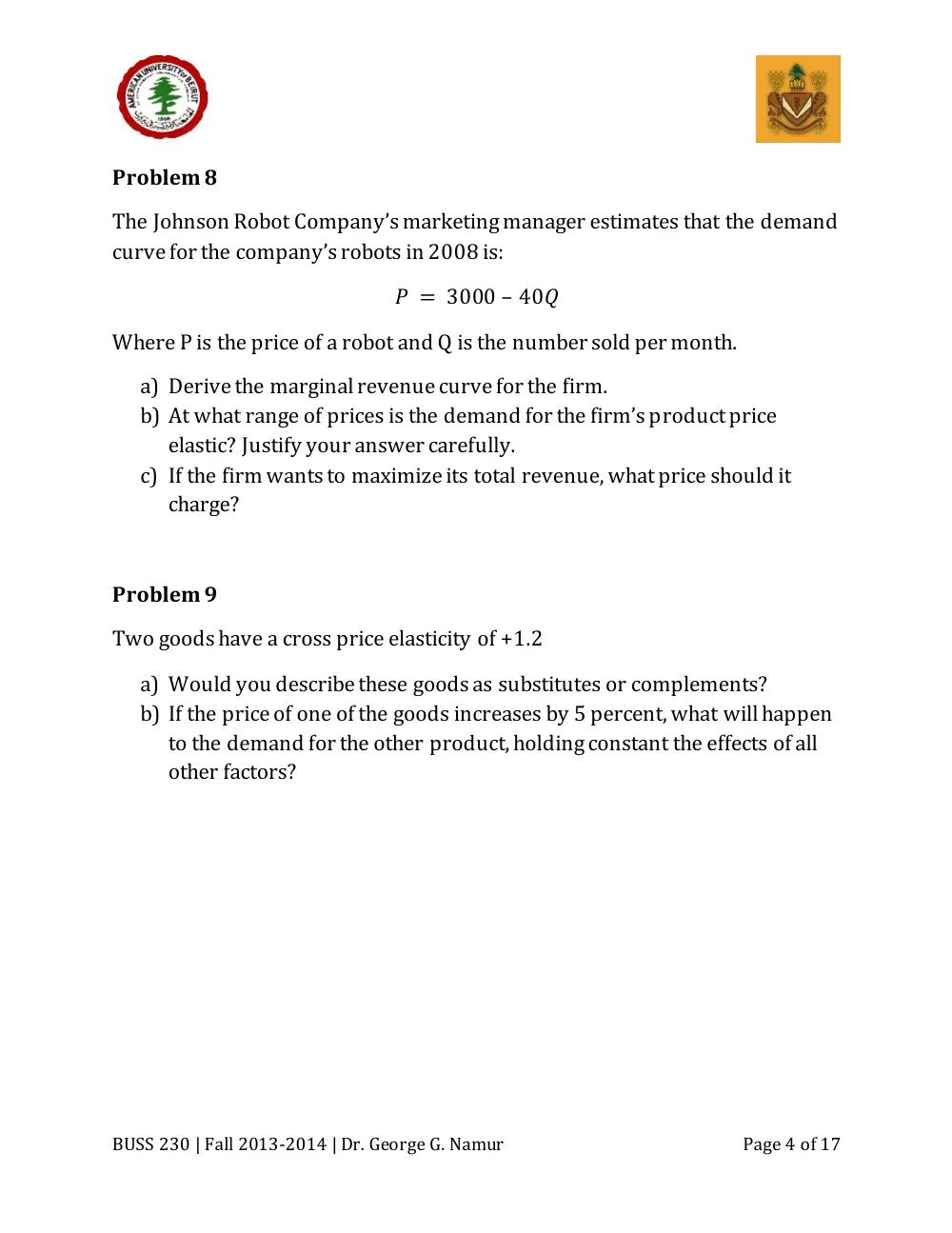Namur Page 4 of 17 Problem 8 The Johnson Robot Company’s marketing manager estimates that the demand curve for the company’s robots in 2008 is: – Where P is the price of a robot and Q is the number sold per month. a) Derive the marginal revenue curve for the firm. b) At what range of prices is the demand for the firm’s product price elastic? Justify your answer carefully. c) If the firm wants to maximize its total revenue, what price should it charge? Problem 9 Two goods have a cross price elasticity of +1.2 a) Would you describe these goods as substitutes or complements? b) If the price of one of the goods increases by 5 percent, what will happen to the demand for the other product, holding constant the effects of all other factors? BUSS 230 | Fall 2013-2014 | Dr. George G. 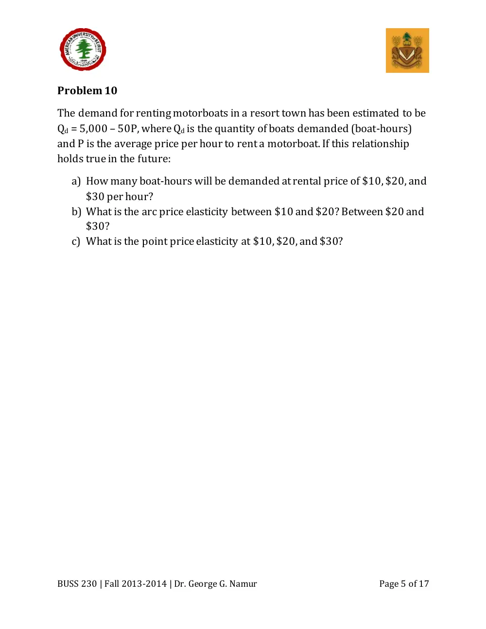Namur Page 5 of 17 Problem 10 The demand for renting motorboats in a resort town has been estimated to be Qd = 5,000 – 50P, where Qd is the quantity of boats demanded (boat-hours) and P is the average price per hour to rent a motorboat. If this relationship holds true in the future: a) How many boat-hours will be demanded at rental price of $10, $20, and $30 per hour? b) What is the arc price elasticity between $10 and $20? Between $20 and $30? c) What is the point price elasticity at $10, $20, and $30? BUSS 230 | Fall 2013-2014 | Dr. George G. 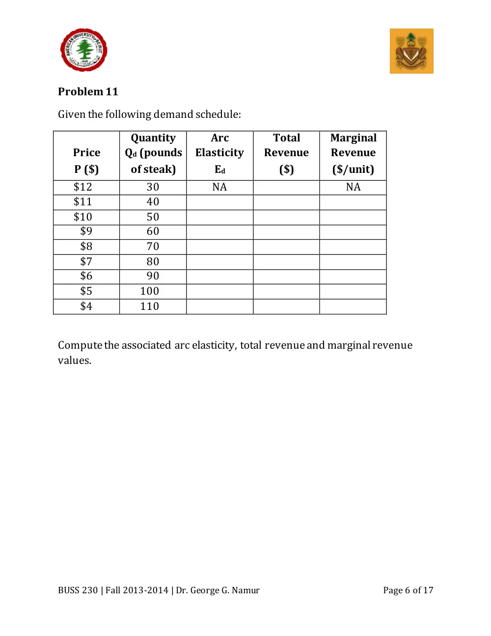Namur Page 6 of 17 Problem 11 Given the following demand schedule: Quantity Arc Total Marginal Price Qd (pounds Elasticity Revenue Revenue P ($) of steak) Ed ($) ($/unit) $12 30 NA NA $11 40 $10 50 $9 60 $8 70 $7 80 $6 90 $5 100 $4 110 Compute the associated arc elasticity, total revenue and marginal revenue values. BUSS 230 | Fall 2013-2014 | Dr. George G. 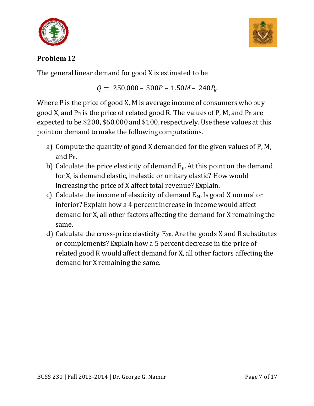Namur Page 7 of 17 Problem 12 The general linear demand for good X is estimated to be – – – Where P is the price of good X, M is average income of consumers who buy good X, and PR is the price of related good R. The values of P, M, and PR are expected to be $200, $60,000 and $100, respectively. Use these values at this point on demand to make the following computations. a) Compute the quantity of good X demanded for the given values of P, M, and PR. b) Calculate the price elasticity of demand Ep. At this point on the demand for X, is demand elastic, inelastic or unitary elastic? How would increasing the price of X affect total revenue? Explain. c) Calculate the income of elasticity of demand EM. Is good X normal or inferior? Explain how a 4 percent increase in income would affect demand for X, all other factors affecting the demand for X remaining the same. d) Calculate the cross-price elasticity EXR. Are the goods X and R substitutes or complements? Explain how a 5 percent decrease in the price of related good R would affect demand for X, all other factors affecting the demand for X remaining the same. BUSS 230 | Fall 2013-2014 | Dr. George G. 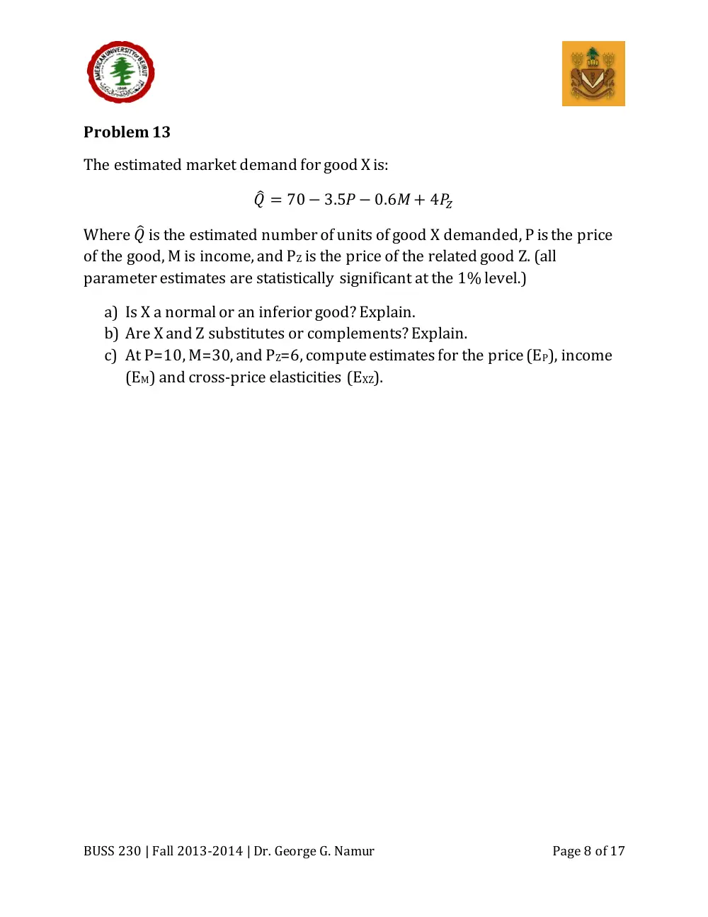Namur Page 8 of 17 Problem 13 The estimated market demand for good X is: ̂ Where ̂ is the estimated number of units of good X demanded, P is the price of the good, M is income, and PZ is the price of the related good Z. (all parameter estimates are statistically significant at the 1% level.) a) Is X a normal or an inferior good? Explain. b) Are X and Z substitutes or complements? Explain. c) At P=10, M=30, and PZ=6, compute estimates for the price (EP), income (EM) and cross-price elasticities (EXZ). BUSS 230 | Fall 2013-2014 | Dr. George G. 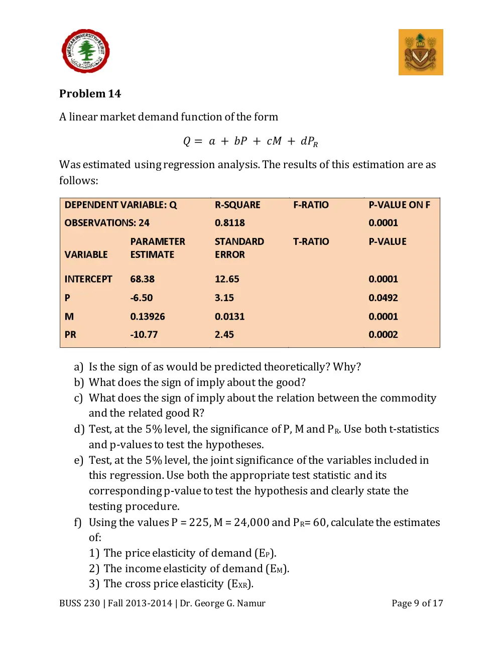Namur Page 9 of 17 Problem 14 A linear market demand function of the form Was estimated using regression analysis. The results of this estimation are as follows: a) Is the sign of as would be predicted theoretically? Why? b) What does the sign of imply about the good? c) What does the sign of imply about the relation between the commodity and the related good R? d) Test, at the 5% level, the significance of P, M and PR. Use both t-statistics and p-values to test the hypotheses. e) Test, at the 5% level, the joint significance of the variables included in this regression. Use both the appropriate test statistic and its corresponding p-value to test the hypothesis and clearly state the testing procedure. f) Using the values P = 225, M = 24,000 and PR= 60, calculate the estimates of: 1) The price elasticity of demand (EP). 2) The income elasticity of demand (EM). 3) The cross price elasticity (EXR). BUSS 230 | Fall 2013-2014 | Dr. George G. Namur Page 10 of 17 Problem 15 Wilpen Company, a price-setting firm, produces nearly 80 percent of all tennis balls purchased in the United States. Wilpen estimates the U.S. 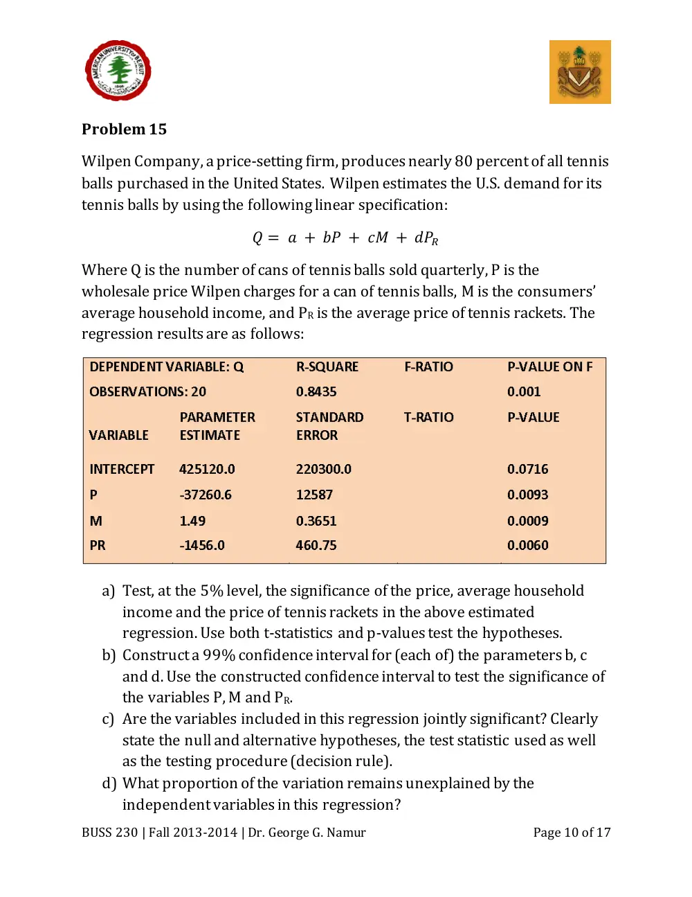demand for its tennis balls by using the following linear specification: Where Q is the number of cans of tennis balls sold quarterly, P is the wholesale price Wilpen charges for a can of tennis balls, M is the consumers’ average household income, and PR is the average price of tennis rackets. The regression results are as follows: a) Test, at the 5% level, the significance of the price, average household income and the price of tennis rackets in the above estimated regression. Use both t-statistics and p-values test the hypotheses. b) Construct a 99% confidence interval for (each of) the parameters b, c and d. Use the constructed confidence interval to test the significance of the variables P, M and PR. c) Are the variables included in this regression jointly significant? Clearly state the null and alternative hypotheses, the test statistic used as well as the testing procedure (decision rule). d) What proportion of the variation remains unexplained by the independent variables in this regression? BUSS 230 | Fall 2013-2014 | Dr. George G. Namur Page 11 of 17 e) Compute the Adjusted R2of this regression. Wilpen plans to charge to charge a wholesale price of $1.65 per can. The average price of a tennis racket is $110, and the consumers’ average household income is $24,600. f) What is the estimated number of cans of tennis balls demanded? g) At the values of P, M and PR given, what are the estimated vales of the price (EP), income (EM), and the cross price elasticity of demand (EXR). h) What will happen, in percentage terms, to the number of cans of tennis balls demanded if the price of tennis balls decreases 15 percent? i) What will happen, in percentage terms, to the number of cans of tennis balls demanded if average household income increases by 20 percent? j) What will happen, in percentage terms, to the number of cans of tennis balls demanded if the average price of tennis rackets increases by 25 percent? BUSS 230 | Fall 2013-2014 | Dr. George G. Namur Page 12 of 17 Problem 16 The estimated market demand for good X is: ̂ where ̂is the estimated number of units of good X demanded, P is the price of good X, M is income, and PG is the price of related good G. (All parameter estimates are statistically significant at the 1 percent level of significance.) a) Is the sign of the coefficient associated with the price consistent with theory? Why or why not? b) Given the above equation, is good X a normal or inferior good? c) Are goods X and G complements or substitutes? d) At P = $12, M = $30,000, and PG = $50, what is the predicted quantity of good X? e) At the values in part (d), compute the following elasticities: 1) Own Price elasticity EP. 2) Cross-price elasticity EXG. 3) Income elasticity EM. f) The R2 from this regression is 0.65. What proportion of the variation in the demand for X is explained by the above regression? What proportion of variation in demand remains unexplained? g) Given a sample size n=25, compute the F-statistic for this demand equation. h) Test, at the 5% level, the joint significance of all the variables included in the regression. i) All else constant, what would be the effect (in percentage terms) of a 20% increase in income? j) All else constant, what would the effect (in percentage terms) of 15% increase in the price of the related product G? BUSS 230 | Fall 2013-2014 | Dr. George G. Namur Page 13 of 17 Problem 17 Rubax, a U.S. manufacturer of athletic shoes, estimates the following linear trend model for shoe sales: Where: Qt = sales of athletic shoes in the quarter t t = 1, 2, …, 28 [2001Q1, 2001Q2, ….,2007Q4] D1 = 1 for the 1st quarter of the year, 0 otherwise D2 = 1 for 2nd quarter of the year, 0 otherwise D3 = 1 for the 3rd quarter of the year, 0 otherwise The regression analysis produces the following results: Observations R-Square 28 0.9651 Variable Parameter Estimate Standard Error Intercept 184500 10310 T 2100 340 D1 3280 1510 D2 6250 2220 D3 7010 1580 BUSS 230 | Fall 2013-2014 | Dr. George G. Namur Page 14 of 17 a) Is there sufficient statistical evidence of an upward trend in shoe sales? b) Do these data indicate a statistically significant seasonal pattern of sales for Rubax shoes? If so, what is the seasonal pattern exhibited by the data? Carefully state the seasonal pattern, if any, and justify your answer. c) Using the estimated forecast equation, forecast sales of Rubax shoes for 2008Q3 and 2009Q2. d) How would you improve this forecast equation? BUSS 230 | Fall 2013-2014 | Dr. George G. Namur Page 15 of 17 Problem 18 A firm experienced the demand shown in the following table: 3-Year Exponential Actual Moving Smoothing Year Demand Average (w = 0.3) 1995 800 NA NA 1996 925 NA 1997 900 NA 1998 1,025 1999 1,150 2000 1,160 2001 1,200 2002 1,150 a) Compute the forecasts based on a 3-year moving average for 1998, 1999, 2000, 2001 and 2002. b) Compute exponential smoothing forecasts of demand using w = 0.3 for 1996, 1997, 1998, 1999, 2000, 2001, 2002. You may begin the exponential smoothing forecasting by assuming that the first forecast value (F1) is equal to the actual (realized) value (A1). c) What criterion would you use to evaluate the accuracy of these forecasts? Write down the expression of the criterion you propose and define the elements of the expression carefully. d) Compute the criterion you propose in part (c) for the 3-year moving average and the exponential smoothing forecasting methods. Which forecasting method does better? BUSS 230 | Fall 2013-2014 | Dr. George G. Namur Page 16 of 17 Problem 19 The demand for tea has been estimated as – Where: Q = thousands of pounds of tea sold P = price per pound of tea I = per capita disposable personal income in thousands of dollars PC = price per pound of coffee a) If next year’s tea price is forecast to be $3, per capita disposable personal income is estimated to be $15,000 (i.e., 15), and the price per pound of coffee is estimated to be $4, compute the expected quantity demanded for the coming year. b) Economic forecasters believe the probability of a major recession next year is high and would reduce per capita income to $13,000 (13). In addition, a frost in Brazil is likely to increase the price of coffee to $7 per round. What impact would these changes in the economic outlook have on the demand for tea? BUSS 230 | Fall 2013-2014 | Dr. George G. Namur Page 17 of 17 Problem 20 Savings-Mart (a chain of discount department stores) sells patio and lawn furniture. Sales are seasonal, with higher sales during the spring and summer quarters and lower sales during the fall and winter quarters. The company developed the following quarterly sales forecasting model: – Where : Ŷt = predicted sales ($million) in quarter t 8.25 = quarterly sales ($ million) when t = 0 t = time period (quarter) where fourth quarter of 2000 = 0, first quarter of 2001 = 1, second quarter of 2001 = 2, … D1 = 1 for first-quarter observations, 0 otherwise D2 = 1 for second-quarter observations, 0 otherwise D3 = 1 for third-quarter observations, 0 otherwise Forecast Savings-Mart’s sales of patio and lawn furniture for each quarter of 2006.