BUSS 230 Midterm, Spring 2004

AMERICAN UNIVERSITY of BEIRUT SCHOOL of BUSINESS BUSS 230 MID-TERM EXAM - March 25, 2004 NAME: ID: SECTION: INSTRUCTOR: ANSWER ALL QUESTIONS ~ TIME ALLOWED: 1 % hours L Multiple choice - (30 points). Please CIRCLE the correct answer 1. Naji earns $50,000 business profit a year by selling donuts. He pays $12,000 a year in rent to his uncle Nabih for the building in which the business is located. If Uncle Nabih gives him the building, then Naji’s a. Business profit will be unchanged. b. Economic profit will be unchanged. Implicit cost will decrease by $12,000 a year. Naji’s revenues will increase by $12,000 a year. All of the above are correct. a aed 2. Implicit cost is equal to: . » Business profit minus economic profit. 3 Business profit plus economic profit. ro Economic profit minus business profit. Economic profit minus explicit costs. Revenues minus explicit costs. pao gp 3. Ifa computer software company introduces a new program and finds that orders from wholesalers far exceed the number of units that are being produced, There is an excess supply and price can be expected to fall. There is an excess supply and price can be expected to rise. There is an excess demand and price can be expected to fall. There is an excess demand and price can be expected to rise. There is a combination of excess demand and supply. eae ge 4. A firm’s revenue function was estimated as TR = 200 Q — 20 Q“2. What would average revenue be when one unit of output is produced? a. 180. b. 160. c. 20. d. 200. e. 220. 5. If marginal revenue is equal to zero, then a. Total revenue is zero. ao m N b. Average revenue is zero. Ge we - j- 10. 11. c. Total profit is at a maximum or minimum. d. Total revenue is at a maximum or a minimum. e. Average revenue is at a maximum or minimum When total revenue is at a maximum: a. Profit is at a maximum. b. Average revenue is at a maximum. / c. Marginal revenue is at a maximum. ~ oY d ; e . Average revenue is equal to zero. . None of the above is correct. The price of a firm’s product increases from $5 to $6. As a result, the quantity demanded of the product declines from 600,000 to 500,000. The price elasticity of demand for the product is equal to: a. -5. b. -3. c. -l. d. -1/3. e. —1/5. If marginal revenue is $20 when the price of the product is $40, then the price elasticity of demand is: a. -2. b. -1. c. - 0.50. d. -0.25. e. 2. If consumer income declines, then the demand for: Normal goods will increase. Inferior goods will increase. The price of the good will increase. Substitute goods will increase. Complementary goods will increase. gagc Tf Application of simple linear regression estimation to sales data yielded the following equation: Q = 24 - 2 P. Ifthe current product price is P = 6 and the quantity sold at that price is Q = 10, then the error (e) for the current time period is: 4, 2. 0. -2. -4. ep agste The adjusted value of the coefficient of determination: a. Will increase if additional independent variables are added to the regression model. -2- Is equal to the proportion of the sum of the squared deviations of the dependent variable from its mean that is explained by the regression model. Is greater than the proportion of the sum of the squared deviations of the dependent variable from its mean that is explained by the regression model. Is smaller than the proportion of the sum of the squared deviations of the dependent variable from its mean that is explained by the regression model. e. Is greater than the unadjusted coefficient of determination. 12. Autocorrelation refers to a situation in which: a. Successive error terms derived from the application of regression estimation to time series data are correlated. b. Successive error terms derived from the application of regression estimation to cross-sectional data are correlated There is a high degree of correlation between two or more of the independent variables included in a multiple regression model. The dependent variable is automatically correlated with the independent variable(s) in a regression model. The application of a multiple regression model yields estimates that are nonlinear in form. 13. Regression was used to estimate the following seasonal forecasting equation: St = 124 + 2.5 T + 18 Di — 46 D2 -28 Ds. Where Diis a dummy variable that is equal to one in the first quarter and zero otherwise, D2 is a dummy variable that is equal to one in the second quarter and zero otherwise, and Ds is a dummy variable that is equal to one in the third quarter and zero otherwise. What would be the forecast for St in the second quarter of time period 10? a. 25.0 b. 95.0 c. 103.0 d. 149.0 e. None of the above is correct. 14. The first step in time-series based forecasting is to: Identify relevant correlated variables. Plot the data on a graph. Calculate a moving average of the observations. Perform preliminary regression calculations. Identify the seasonal pattern in the observations. 15. The use of a smoothing technique is appropriate when: Random behavior is the primary source of variation. Seasonality is present. Data indicate the presence of cyclical fluctuations. Data exhibit a minor downward trend. Data exhibit a minor upward trend. - 3. 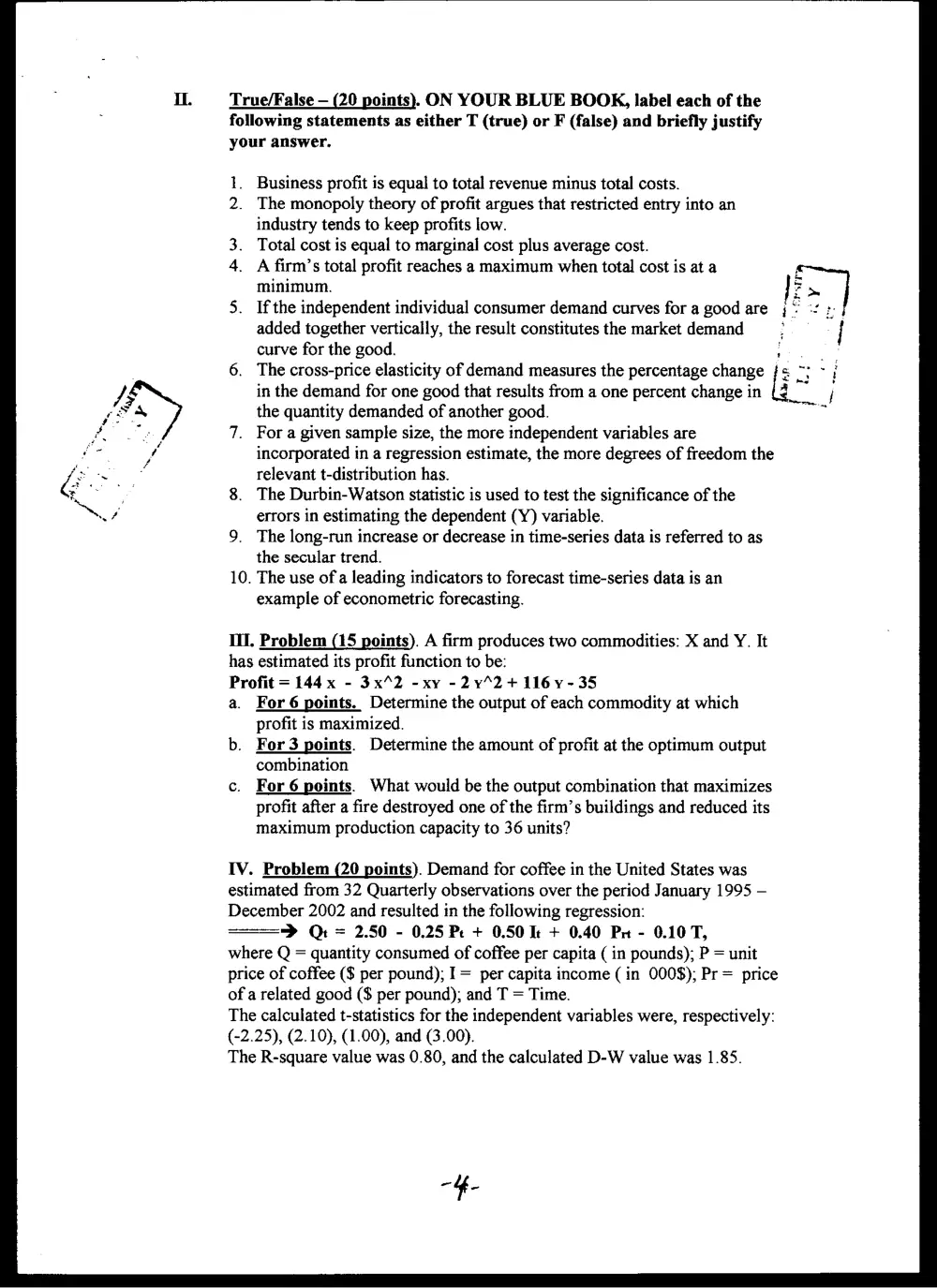IL. True/False — (20 points). ON YOUR BLUE BOOK, label each of the following statements as either T (true) or F (false) and briefly justify your answer. 1. Business profit is equal to total revenue minus total costs. 2. The monopoly theory of profit argues that restricted entry into an industry tends to keep profits low. 3. Total cost is equal to marginal cost plus average cost. 4. A firm’s total profit reaches a maximum when total cost is at a minimum. ° 5. Ifthe independent individual consumer demand curves for a good are ; °° :: added together vertically, the result constitutes the market demand ; | curve for the good. mol 6. The cross-price elasticity of demand measures the percentage change {= 7; ~ i in the demand for one good that results from a one percent change in [i> the quantity demanded of another good. 7. Fora given sample size, the more independent variables are incorporated in a regression estimate, the more degrees of freedom the relevant t-distribution has. 8. The Durbin-Watson statistic is used to test the significance of the errors in estimating the dependent (Y) variable. 9. The long-run increase or decrease in time-series data is referred to as the secular trend. 10. The use of a leading indicators to forecast time-series data is an example of econometric forecasting. oad III. Problem (15 points). A firm produces two commodities: X and Y. It has estimated its profit function to be: Profit = 144 x - 3x42 -xy -2y°2+ 116 y-35 a. For6 points. Determine the output of each commodity at which profit is maximized. b. For 3 points. Determine the amount of profit at the optimum output combination c. For 6 points. What would be the output combination that maximizes profit after a fire destroyed one of the firm’s buildings and reduced its maximum production capacity to 36 units? IV. Problem (20 points). Demand for coffee in the United States was estimated from 32 Quarterly observations over the period January 1995 — December 2002 and resulted in the following regression: > Qt = 2.50 - 0.25 Pr + 0.50 It + 0.40 Pr - 0.10 T, where Q = quantity consumed of coffee per capita ( in pounds); P = unit price of coffee ($ per pound); I= per capita income (in 000$); Pr = price of a related good ($ per pound); and T = Time. The calculated t-statistics for the independent variables were, respectively: (-2.25), (2.10), (1.00), and (3.00). The R-square value was 0.80, and the calculated D-W value was 1.85. 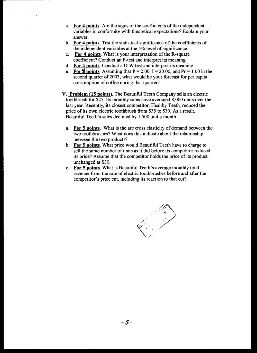a. For 4 points. Are the signs of the coefficients of the independent variables in conformity with theoretical expectations? Explain your answer. b. For 4 points. Test the statistical significance of the coefficients of the independent variables at the 5% level of significance. c. For 4 points. What is your interpretation of the R-square coefficient? Conduct an F-test and interpret its meaning. d. For 4 points. Conduct a D-W test and interpret its meaning. e. For points. Assuming that P = 2.00, I = 20.00, and Pr = 1.00 in the second quarter of 2003, what would be your forecast for per capita consumption of coffee during that quarter? V. Problem (15 points). The Beautiful Teeth Company sells an electric toothbrush for $25. Its monthly sales have averaged 8,000 units over the last year. Recently, its closest competitor, Healthy Teeth, reduced the price of its own electric toothbrush from $35 to $30. As a result, Beautiful Teeth’s sales declined by 1,500 unit a month. a. For 5 points. What is the arc cross elasticity of demand between the two toothbrushes? What does this indicate about the relationship between the two products? b. For 5 points. What price would Beautiful Teeth have to charge to sell the same number of units as it did before its competitor reduced its price? Assume that the competitor holds the price of its product unchanged at $30. c. For 5 points. What is Beautiful Teeth’s average monthly total revenue from the sale of electric toothbrushes before and after the competitor’s price cut, including its reaction to that cut? 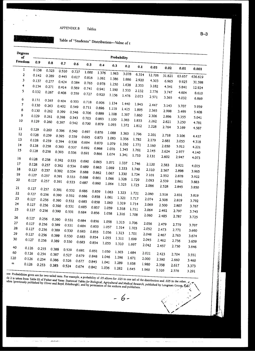APPENDIX B Tables Pek ey Table of “Students” Distribution—Value of t Probability 0.7 0.325 0.510 0.289 0,445 0.277 0,424 0.271 0,414 0.267 0.408 0.265 0.404 0.263 0.402 0.262 0.399 0.261 0.398 0.260 0,397 0.260 0.396 0.259 0,395 0.259 0.394 0.258 0.393 0.258 0.393 0.258 0.392 0.257 0,392 0.257 0.392 0.257 0.391 0.257 0.391 0.257 0.391 0.256 0.390 0.256 0.390 0.256 0.390 0.256 0.390 0.256 0.390 0.256 0.389 0.256 0.389 0.256 0.389 0.256 0.389 0.255 0.388 0.254 0.387 0.254 0.386 0.253 0.385 00'T CCT wet 6€T 9bT wt “2st L9T Sit €8T S881 +6T WC OZ We L4E~T O97 COOL HE STI SET ey Ost Sst I9T 99°T SLT eet I6T 96% OT GOT LTT 6% SHT BOT LOE CWE OV 6fT LyT ST 66T SOT O21 SLT ST TOT 661 POT OTT LTT STZ LET EST O4T STE OOF 09 I¢T 8ST OT 69T FLT 6LZT +8 6T O07 807 %~@Z SIT STZ HET SHT 197 BZ ETE BOF OF wT 89'T oLT 6L1T = +8T 68'T £6T Ot 60% 91 It L477 ECT CHT EST 697 WU EE LTb Of v9OT oLT GLY Wl Sst O6T r6T €OT O1Z BIZ We BC SET EFT GET OLT 6% €C£ Blb 62% SOT ZT 242%) 78T L8T I6T 96T 0% ZIZ GTZ FT GTC ET SHE 9ST Wt SOT FEE OTH 87 LOT eZ T 6LT +8T sel €6T L461 907 €1% O77 SZ tet LET OFF LET ELT 967 SEE Itb 17 69T SLT 0s'T set O67 S6T 66T 207 Stt Ut LOT TT CEC LOT GET HLT B67 LEE Th ZT LLY 781 481 76'T 961 ot 60% OTT POT BCT HEC OFC GHZ «(OOF «(OOLT BHT 6E€ bh elt 6LT $8'T 68T +6'T 861 £07 ITZ 8T@ StT OCT DET WT Ist %@9Z 8L% OE OE OH Fz OLT Ist 98'T T6T 96°T TOT «SOT ETT OCT LT TET LET HHT EST HOT OBZ COE WE Bb sit $81 68st +461 86T OT LOT STT €@7 OFZ FEZ OKT OFZ SET 99T WE SOE HE OFh TW T8'T A8°T TOT 96°T TOT SOT OTT BIZ SCT TET LET Wl 6HT LET BOT HBT LOE LE tee Tt +81 06'T S6T 661 +07 807 It OTT BZ SET GEV. SHZ Ist 09% Lt L287 OTE GFE Sob 07 88'T £6T 86T OT L0t 1% OTT €7T Tet «BET MHC BHT OST OENTOLT COHTSCET'E:SCO UGE BEOCT tOT L6°T wT «090% —OTT?R STE OTT OLUT CO HET OWT OCOOHZOIGZ «BST ODT Ss LLT SCEHTCOOT'E. soe Ihe 81 1 96T loz 90% O17 STITT 617% €tZ TEC BEC SHC GHZ SS7 19% = OL'T 187 96% OTE 69E wr Lt ian 107 90°F IT? STt 61 FC BCT SET THT OORT OT OST ODT SHA TCGBIZ WE +e CE 6kr 9T LOT ITZ 9TT OCT STU 6ct «EC (OWT BHT OST OST HOT et 6LT O67 OE 6TE BOE Be Ct \ £1T STZ TC Let EZ SET 6€T OFC EST O9T SOT OLT BLT SBT 9T ITE HEE FHLE 09F FI ITZ St? Of FET BET CHE BT EST OFF 49% ILE LLT €CB% WF COE BIE IKE T8€ Lob eT O€T = =FET BET EFT Let St 8% TC 69T SLT O8T SBT 167 00°€ WE OE GRE 6RE Sle tT & Or? SoZ 6F~ EST LST 19% S97 Wt 6£7 SBT O67 S67 Toe GOE OTE BEE 6SE B6E HF a & $S7 8ST TT 99T «=—OLT OLE LET OST 167 862 WE LOE PIE (WE CCE BE ILE Ob 96% OF Ut SLT 6L7 €B87T 98 O6C +67 TOE L40€ PTE BITE ETE OTE LEE BE EC9E OBE OTH TTS 6 i. £67 L167 Toe s0€ BOF CIE STE CE BIE SEE GEE HE OSE BOE G69E HE LO OF ES 8 a ete LTE OCC FEE BEE Ire tre TSE LSE +9E BOE ELE GLE LWE L6E Wh %GEb Hey 6ss o£ Fa ge oe +2€ “L4ee I8€ +8E LE FOE OOF 906 OTh STb Th 8b Geb €Sb Db FITS 66'S 9 & 9b Obb fhe Ob OSb ESb bh Cb BOF tle Llb Whe B8b S6b SOS 61S WS 6L¢ 199 S * O'S 9¢o 8669S) TLE OLS 4bE 08S) OBS: TGS «—OBE 0D 409 609 OTD OTD HED «66S DBD Zh + ess sc8 498 698 7S +198 998 O48 +48 6L48 I88 S88 688 +68 106 ZI6 876 SS6 €10I £€ OS61 G6r6T 8F6l Le6l OF6I ShOl Sh6I €H6I TH6T OF61 SET LEGT SESI ECE6T OLGT S76I OF6I OO6T ZERI 7 erse €€SC CT7SC TISt TOS T6et O8bl GST GEbZ GIT LOT GRET BOET OFEZ COZ OF7Z LSIZ SE6l FH I9T I © 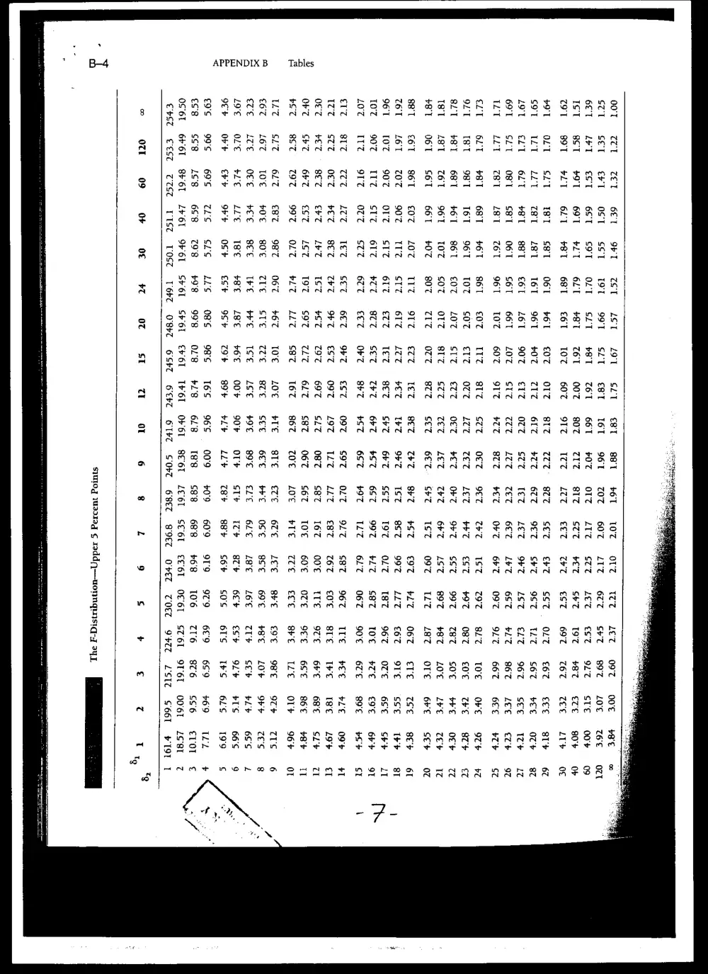id § 09 OF of <4 0t St a ot 6 8 L 9 s + € c T 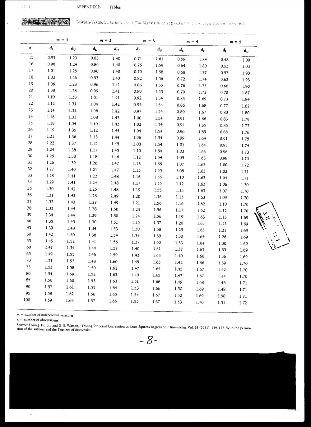APPENDIX B Tables Tawoin We m=1 m= m=3 m= 4 m=5 nt a, dy a, dy a dy da, dy d, dy 15095 123 0.83 140. O71 L6l~(059~—~*«d«B4SCABWSS*~«a 16 0.98 1.24 0.86 1.40 0.75 159 0.64 1.80 0.53 2.03 WW LOL 1.25 0.90 1.40 0.79 1.58 0.68 LI7 0.57 1.98 18 1.03 1.26 0.93 1.40 0.82 1.56 0.72 174 0.62 1.93 19 1.06 1.28 0.96 L41 0.86 155 0.76 LB 0.66 1.90 20 1.08 1.28 0.99 141 0.89 155 0.79 1.72 0.70 1.87 21 1.10 1.30 1.01 L4l 0.92 1.54 0.83 1.69 0.73 1.84 2 112 131 1.04 1.42 0.95 154 0.86 1.68 0.77 1.82 23 Lid 1.32 1.06 1.42 0.97 1.54 0.89 1.67 0.80 1.80 4 1.16 1.33 1.08 1.43 1.00 154 0.91 1.66 0.83 1.79 25 118 1.34 1.10 1.43 1.02 1.54 0.94 1.65 0.86 77 26 119 1.35 L12 1.44 1.04 154 0.96 1.65 0.88 L.76 27 121 1.36 113 1.44 1.06 154 0.99 1.64 0.91 L75 28 1.22 1.37 LAs 1.45 1.08 154 1.01 1.64 0.93 L.74 29 1.24 1.38 LW 1.45 1.10 L34 1,03 1.63 0.96 LB 30 1.25 1.38 1.18 1.46 112 1.54 1.05 1.63 0.98 L73 31 1.26 1.39 1.20 LAT LB 1.55 1.07 1.63 1.00 L7?2 32 127 1.40 1.22 147 115 155 1.08 1.63 1.02 L71 33 1.28 Lal 1.22 1.48 1.16 1.55 1.10 1.63 1.04 71 34 1.29 L4l 1.24 1.48 117 155 112 1.63 1.06 1.70 35 130 1.42 1.25 1.48 1.19 155 LB 1.63 1.07 1.70 36 131 1.43 1.26 1.49 1.20 1.56 Ls 1.63 1.09 1.70 37 132 1.43 1.27 1.49 121 1.56 1.16 1.62 1.10 1.70 38 133 1.44 1.28 1.50 1.23 1.56 L17 1.62 LW 1.70 39 134 1.44 1.29 1.50 1.24 1.56 1.19 1.63 113 1.69 40 135 145 1.30 151 1.25 157 1.20 1.63 115 1.69 45 139 1.48 1.34 1.53 1.30 1.58 1.25 1.63 1.21 1.69 50 142 1.50 1.38 1.54 1.34 159 1.30 1.64 1.26 1.69 55 145 1.52 Lat 1.56 1.37 1.60 1.33 1.64 1.30 1.69 60 LaT 1.54 1.44 1.57 1.40 161 137 1.65 1.33 1.69 65 1.49 1.55 1.46 1.59 1.43 1.63 1.40 1.66 1.36 1.69 70 151 157 1.48 1.60 1.45 1.63 142 1.66 1.39 1.70 75 1.53 1.58 1.50 1.61 L47 1.64 145 1.67 1.42 1.70 80 154 1.59 1.52 1.63 1.49 1.65 La7 1.67 La4 1.70 85 1.56 1.60 153 1.63 151 1.66 1.49 1.68 1.46 L71 90 157 161 1.35 1.64 1.53 1.66 1.50 1.69 1.48 wal 95 1.58 1.62 1.56 1.65 154 1.67 1.52 1.69 1.50 L71 100 159 1.63 1.57 1.65 1.55 1.67 1.53 1.70 151 L72 m = number of independent variables n = number of observations Source: From J. Durbin and G. S. Watson, “Testing for Serial Correlation in Least-Squares Regression,” Biometrika, Vol. 38 (1951): 159-177. With the permis- sion of the authors and the Trustees of Biometrika. ~ B-