CMPS 251 Problems Practice (Chapter 4), Fall 2015

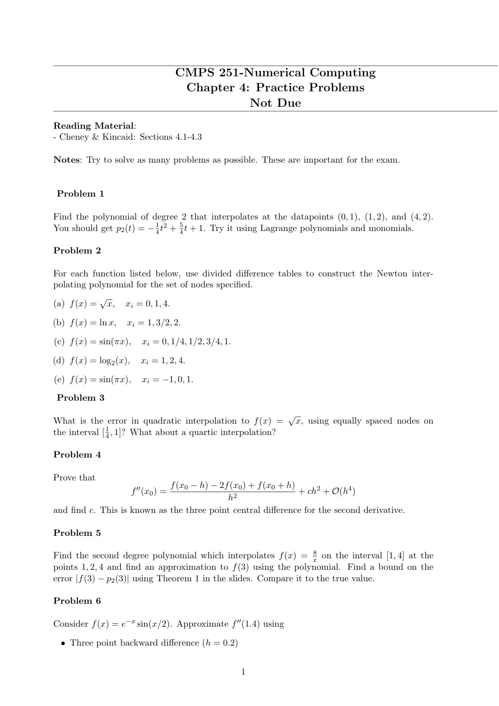
CMPS 251-Numerical Computing Chapter 4: Practice Problems Not Due Reading Material: - Cheney & Kincaid: Sections 4.1-4.3 Notes: Try to solve as many problems as possible. These are important for the exam. Problem 1 Find the polynomial of degree 2 that interpolates at the datapoints (0, 1), (1, 2), and (4, 2). You should get p2(t) = − 1 4t2 + 5 4t + 1. Try it using Lagrange polynomials and monomials. Problem 2 For each function listed below, use divided difference tables to construct the Newton inter- polating polynomial for the set of nodes specified. (a) f(x) = √x, xi = 0, 1, 4. (b) f(x) = ln x, xi = 1, 3/2, 2. (c) f(x) = sin(πx), xi = 0, 1/4, 1/2, 3/4, 1. (d) f(x) = log2(x), xi = 1, 2, 4. (e) f(x) = sin(πx), xi = −1, 0, 1. Problem 3 What is the error in quadratic interpolation to f(x) = √x, using equally spaced nodes on the interval [ 1 4, 1]? What about a quartic interpolation? Problem 4 Prove that f′′(x0) = f(x0 − h) − 2f(x0) + f(x0 + h) h2 + ch2 + O(h4) and find c. This is known as the three point central difference for the second derivative. Problem 5 Find the second degree polynomial which interpolates f(x) = 8 x on the interval [1, 4] at the points 1, 2, 4 and find an approximation to f(3) using the polynomial. Find a bound on the error |f(3) − p2(3)| using Theorem 1 in the slides. Compare it to the true value. Problem 6 Consider f(x) = e−x sin(x/2). 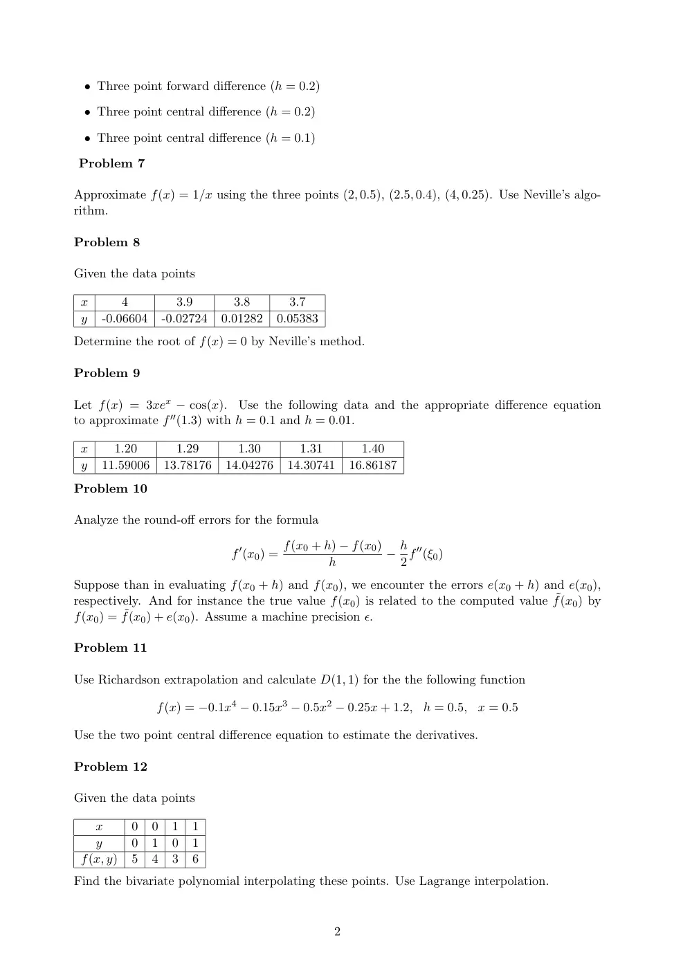Approximate f′′(1.4) using • Three point backward difference (h = 0.2) 1 • Three point forward difference (h = 0.2) • Three point central difference (h = 0.2) • Three point central difference (h = 0.1) Problem 7 Approximate f(x) = 1/x using the three points (2, 0.5), (2.5, 0.4), (4, 0.25). Use Neville’s algo- rithm. Problem 8 Given the data points x 4 3.9 3.8 3.7 y -0.06604 -0.02724 0.01282 0.05383 Determine the root of f(x) = 0 by Neville’s method. Problem 9 Let f(x) = 3xex − cos(x). Use the following data and the appropriate difference equation to approximate f′′(1.3) with h = 0.1 and h = 0.01. x 1.20 1.29 1.30 1.31 1.40 y 11.59006 13.78176 14.04276 14.30741 16.86187 Problem 10 Analyze the round-off errors for the formula f′(x0) = f(x0 + h) − f(x0) h − h 2f′′(ξ0) Suppose than in evaluating f(x0 + h) and f(x0), we encounter the errors e(x0 + h) and e(x0), respectively. And for instance the true value f(x0) is related to the computed value ˜f(x0) by f(x0) = ˜f(x0) + e(x0). Assume a machine precision ϵ. Problem 11 Use Richardson extrapolation and calculate D(1, 1) for the the following function f(x) = −0.1x4 − 0.15x3 − 0.5x2 − 0.25x + 1.2, h = 0.5, x = 0.5 Use the two point central difference equation to estimate the derivatives. Problem 12 Given the data points x 0 0 1 1 y 0 1 0 1 f(x, y) 5 4 3 6 Find the bivariate polynomial interpolating these points. Use Lagrange interpolation. 2 Problem 13 Find an approximation to f′(x1) by differentiating the quadratic polynomial which interpo- lates f at the points x0 = x1 − h1, x1, x2 = x1 + h2. What does the formula reduce to when h1 = h2 = h? 3