CMPS 251 Homework Assignment 3, Fall 2015

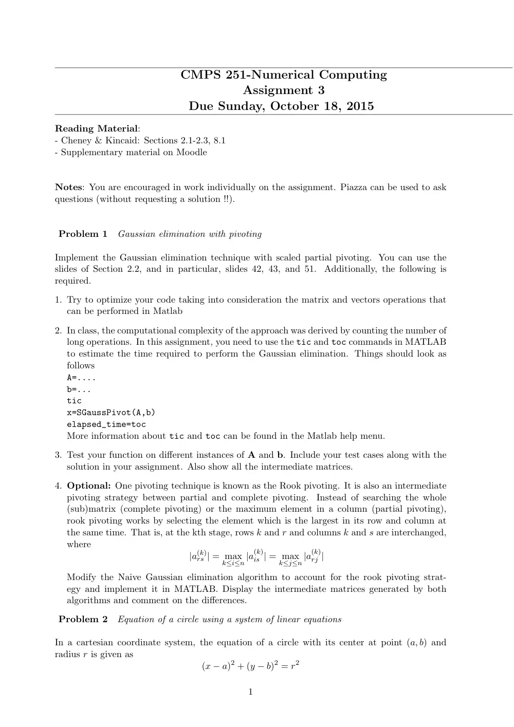
CMPS 251-Numerical Computing Assignment 3 Due Sunday, October 18, 2015 Reading Material: - Cheney & Kincaid: Sections 2.1-2.3, 8.1 - Supplementary material on Moodle Notes: You are encouraged in work individually on the assignment. Piazza can be used to ask questions (without requesting a solution !!). Problem 1 Gaussian elimination with pivoting Implement the Gaussian elimination technique with scaled partial pivoting. You can use the slides of Section 2.2, and in particular, slides 42, 43, and 51. Additionally, the following is required. 1. Try to optimize your code taking into consideration the matrix and vectors operations that can be performed in Matlab 2. In class, the computational complexity of the approach was derived by counting the number of long operations. In this assignment, you need to use the tic and toc commands in MATLAB to estimate the time required to perform the Gaussian elimination. Things should look as follows A=.... b=... tic x=SGaussPivot(A,b) elapsed_time=toc More information about tic and toc can be found in the Matlab help menu. 3. Test your function on different instances of A and b. Include your test cases along with the solution in your assignment. Also show all the intermediate matrices. 4. Optional: One pivoting technique is known as the Rook pivoting. It is also an intermediate pivoting strategy between partial and complete pivoting. Instead of searching the whole (sub)matrix (complete pivoting) or the maximum element in a column (partial pivoting), rook pivoting works by selecting the element which is the largest in its row and column at the same time. That is, at the kth stage, rows k and r and columns k and s are interchanged, where |a(k) rs | = max k≤i≤n |a(k) is | = max k≤j≤n |a(k) rj | Modify the Naive Gaussian elimination algorithm to account for the rook pivoting strat- egy and implement it in MATLAB. Display the intermediate matrices generated by both algorithms and comment on the differences. Problem 2 Equation of a circle using a system of linear equations In a cartesian coordinate system, the equation of a circle with its center at point (a, b) and radius r is given as (x − a)2 + (y − b)2 = r2 1 Given three points, we need to determine the equation of a circle that passes through these points. Let these points have the coordinates (α1, β1), (α2, β2), and (α3, β3), respectively. One way to solve the problem is to transform it into a system of linear equations. To this end, you need to define your equations with the appropriate variables (hint: these are functions of a, b and r). 1. Derive the system of equations and write it in the form Ax = b 2. Solve the equation using Gaussian elimination by hand for the following points: (−1, 3.2), (−8, 4), and (−6.5, −9.3) 3. Check your solution using Matlab’s A\b Problem 3 Ill-Conditioned Matrices Consider the following system of equations { 34.9x1 + 23.6x2 = 234 22.9x1 + 15.6x2 = 154 1. Solve this system with your technique of choice 2. Change the first coefficient of x1 to 35.0 and the second coefficient of x1 to 22.8. Also, change the first constant term to 235. Solve the system again and comment on the differences. 3. Compute the infinity condition number of the original matrix A by forming A, computing its inverse A−1 and caculating the infinity norms ||A||∞, and ||A−1||∞. Comment on the obtained value. Estimate the number of digits that you expect to lose when solving Ax = b. 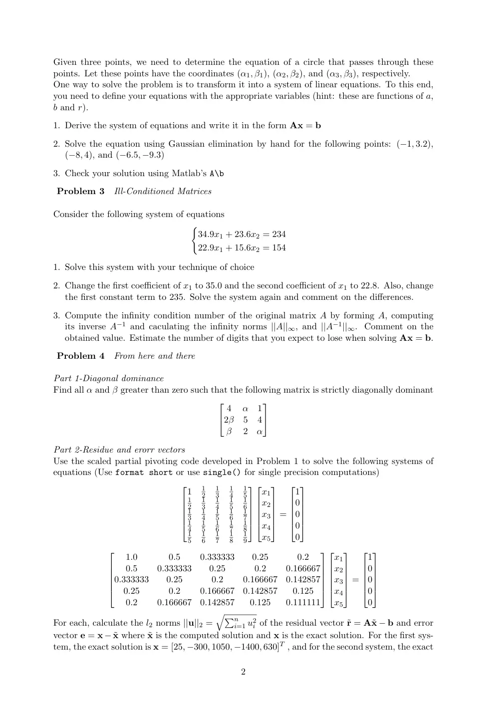Problem 4 From here and there Part 1-Diagonal dominance Find all α and β greater than zero such that the following matrix is strictly diagonally dominant   4 α 1 2β 5 4 β 2 α   Part 2-Residue and erorr vectors Use the scaled partial pivoting code developed in Problem 1 to solve the following systems of equations (Use format short or use single() for single precision computations)   1 1 2 1 3 1 4 1 5 1 2 1 3 1 4 1 5 1 6 1 3 1 4 1 5 1 6 1 7 1 4 1 5 1 6 1 7 1 8 1 5 1 6 1 7 1 8 1 9     x1 x2 x3 x4 x5   =   1 0 0 0 0     1.0 0.5 0.333333 0.25 0.2 0.5 0.333333 0.25 0.2 0.166667 0.333333 0.25 0.2 0.166667 0.142857 0.25 0.2 0.166667 0.142857 0.125 0.2 0.166667 0.142857 0.125 0.111111     x1 x2 x3 x4 x5   =   1 0 0 0 0   For each, calculate the l2 norms ||u||2 = √∑n i=1 u2 i of the residual vector ˜r = A˜x − b and error vector e = x − ˜x where ˜x is the computed solution and x is the exact solution. For the first sys- tem, the exact solution is x = [25, −300, 1050, −1400, 630]T , and for the second system, the exact 2 solution, to six decimal digits of accuracy, is x = [26.9314, −336.018, 1205.11, −1634.03, 744.411]T . Do not change the input data of the second system to include more than the number of digits shown. Analyze the results. What have you learned? Problem 5 Factorizations !!!!! 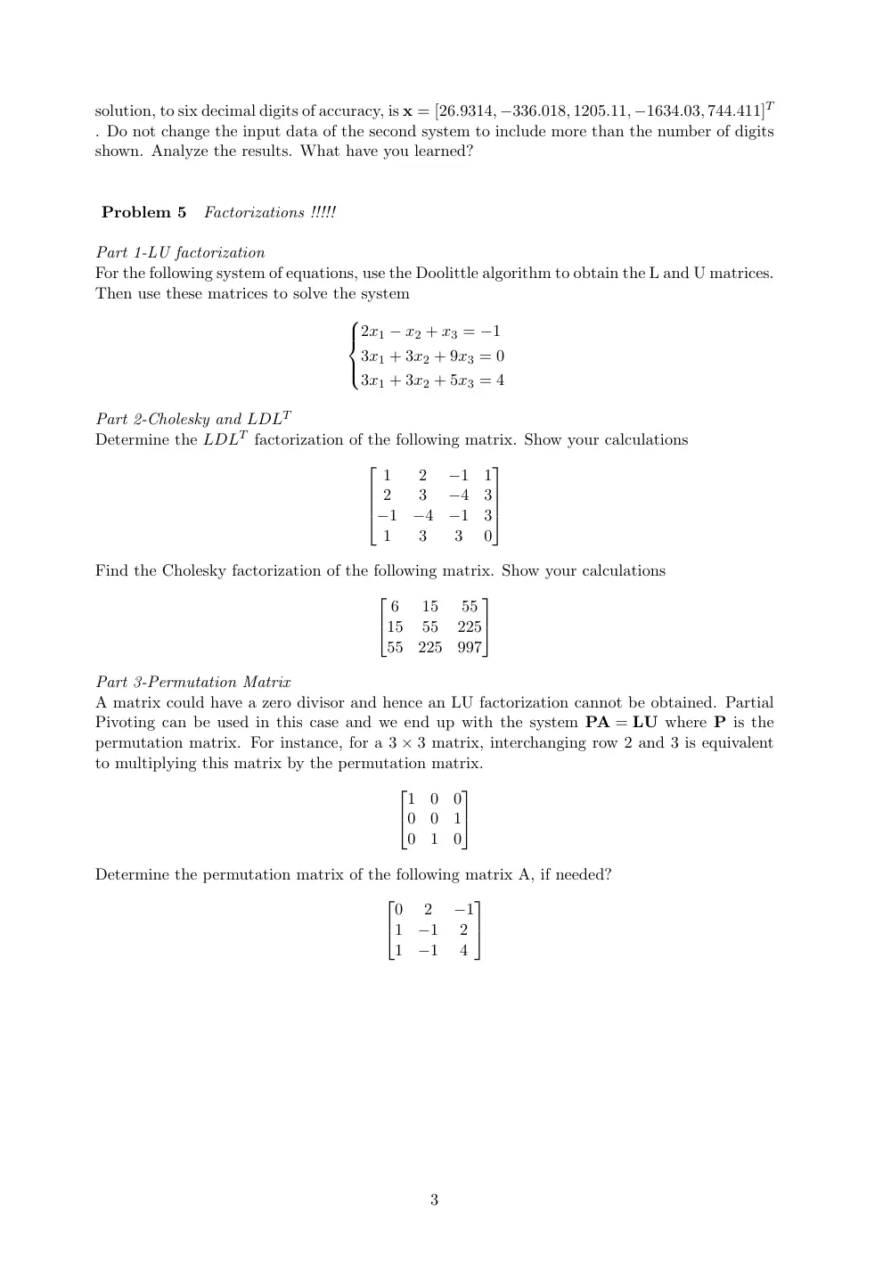Part 1-LU factorization For the following system of equations, use the Doolittle algorithm to obtain the L and U matrices. Then use these matrices to solve the system      2x1 − x2 + x3 = −1 3x1 + 3x2 + 9x3 = 0 3x1 + 3x2 + 5x3 = 4 Part 2-Cholesky and LDLT Determine the LDLT factorization of the following matrix. Show your calculations   1 2 −1 1 2 3 −4 3 −1 −4 −1 3 1 3 3 0   Find the Cholesky factorization of the following matrix. Show your calculations   6 15 55 15 55 225 55 225 997   Part 3-Permutation Matrix A matrix could have a zero divisor and hence an LU factorization cannot be obtained. Partial Pivoting can be used in this case and we end up with the system PA = LU where P is the permutation matrix. For instance, for a 3 × 3 matrix, interchanging row 2 and 3 is equivalent to multiplying this matrix by the permutation matrix.   1 0 0 0 0 1 0 1 0   Determine the permutation matrix of the following matrix A, if needed?   0 2 −1 1 −1 2 1 −1 4   3