CMPS 251 Homework Assignment 1, Fall 2015

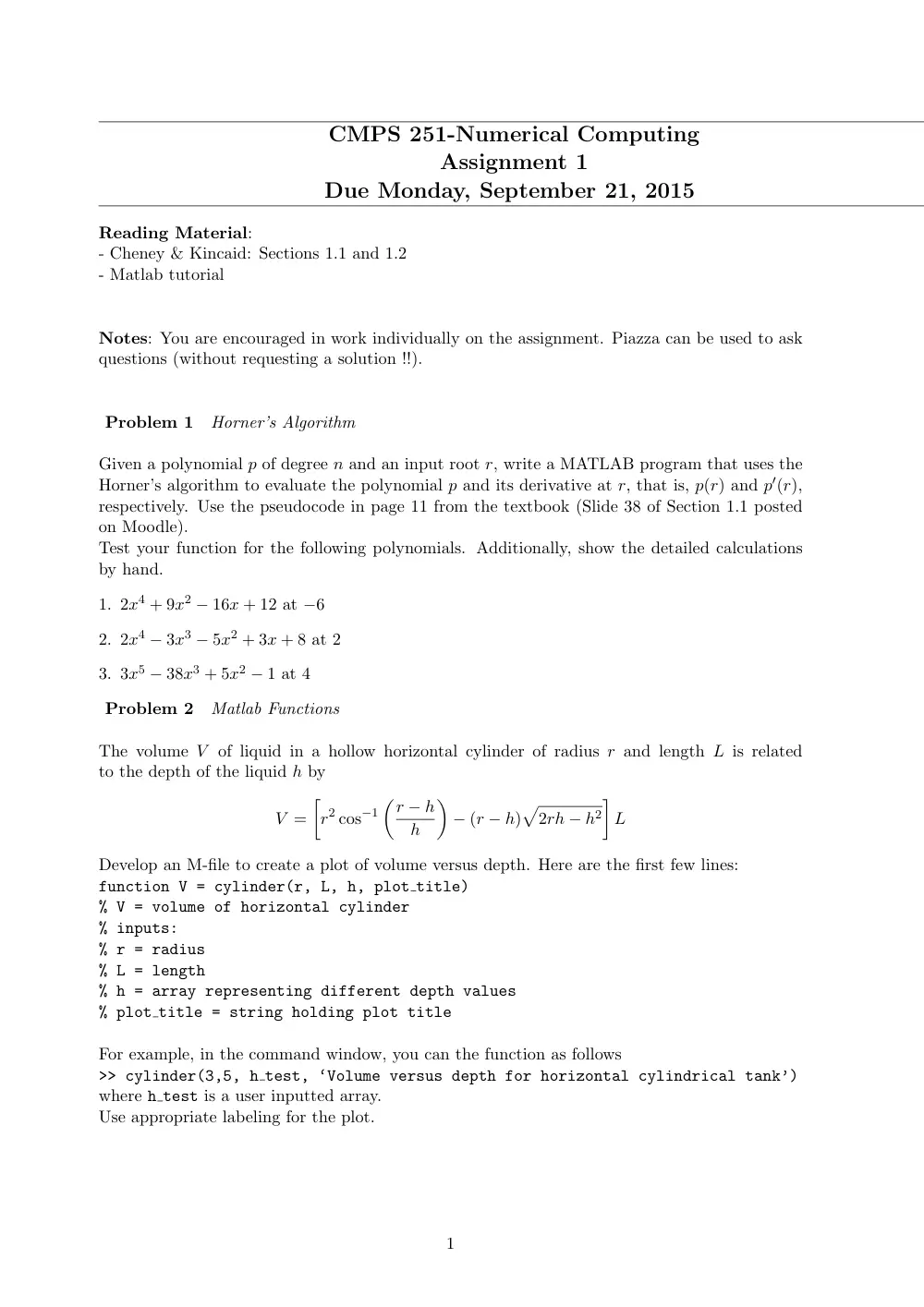
CMPS 251-Numerical Computing Assignment 1 Due Monday, September 21, 2015 Reading Material: - Cheney & Kincaid: Sections 1.1 and 1.2 - Matlab tutorial Notes: You are encouraged in work individually on the assignment. Piazza can be used to ask questions (without requesting a solution !!). Problem 1 Horner’s Algorithm Given a polynomial p of degree n and an input root r, write a MATLAB program that uses the Horner’s algorithm to evaluate the polynomial p and its derivative at r, that is, p(r) and p′(r), respectively. Use the pseudocode in page 11 from the textbook (Slide 38 of Section 1.1 posted on Moodle). Test your function for the following polynomials. Additionally, show the detailed calculations by hand. 1. 2x4 + 9x2 − 16x + 12 at −6 2. 2x4 − 3x3 − 5x2 + 3x + 8 at 2 3. 3x5 − 38x3 + 5x2 − 1 at 4 Problem 2 Matlab Functions The volume V of liquid in a hollow horizontal cylinder of radius r and length L is related to the depth of the liquid h by V = [ r2 cos−1 (r − h h ) − (r − h) √ 2rh − h2 ] L Develop an M-file to create a plot of volume versus depth. Here are the first few lines: function V = cylinder(r, L, h, plot title) % V = volume of horizontal cylinder % inputs: % r = radius % L = length % h = array representing different depth values % plot title = string holding plot title For example, in the command window, you can the function as follows >> cylinder(3,5, h test, ‘Volume versus depth for horizontal cylindrical tank’) where h test is a user inputted array. Use appropriate labeling for the plot. 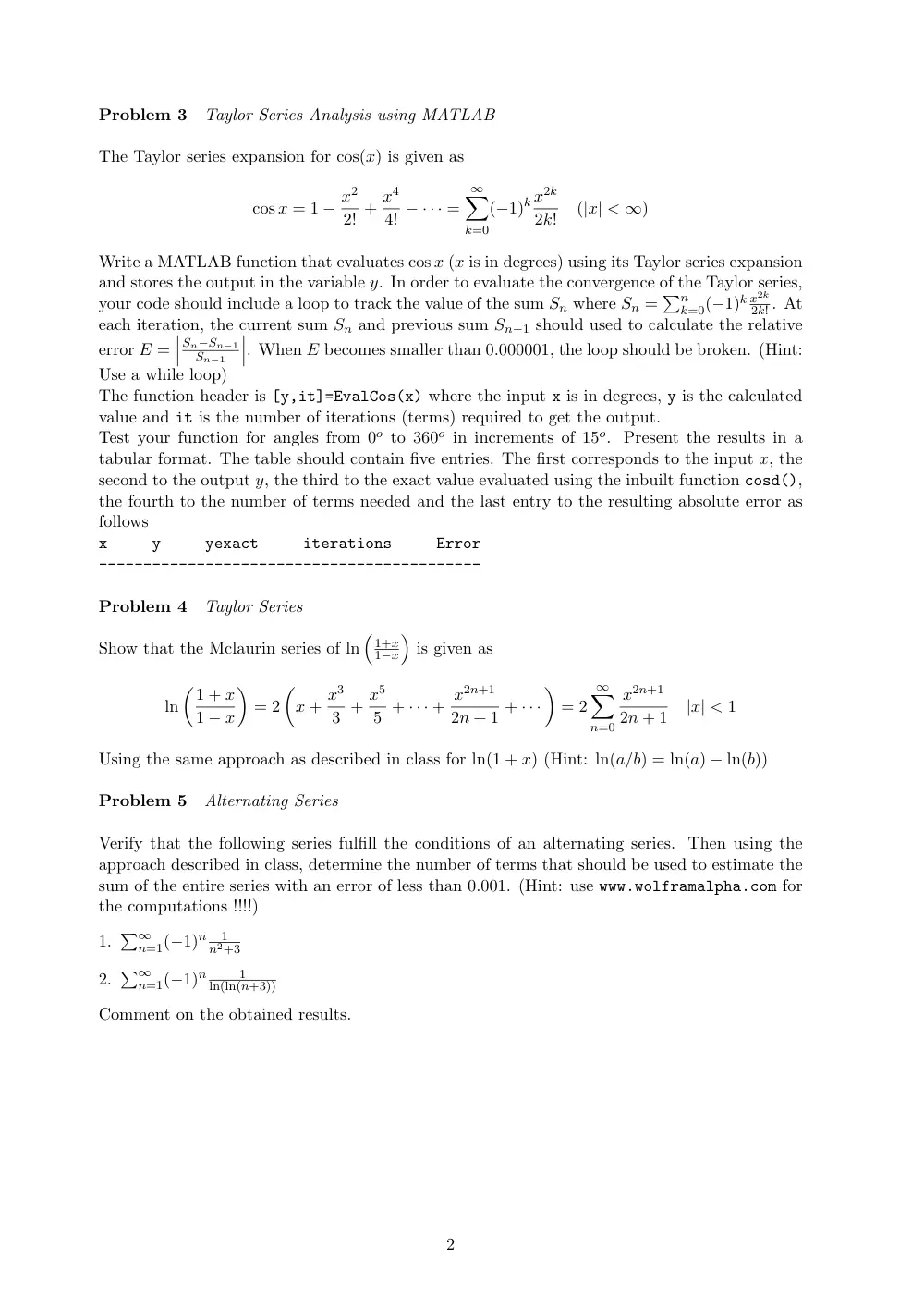1 Problem 3 Taylor Series Analysis using MATLAB The Taylor series expansion for cos(x) is given as cos x = 1 − x2 2! + x4 4! − · · · = ∞ ∑ k=0 (−1)k x2k 2k! (|x| < ∞) Write a MATLAB function that evaluates cos x (x is in degrees) using its Taylor series expansion and stores the output in the variable y. In order to evaluate the convergence of the Taylor series, your code should include a loop to track the value of the sum Sn where Sn = ∑n k=0(−1)k x2k 2k! . At each iteration, the current sum Sn and previous sum Sn−1 should used to calculate the relative error E = ��� Sn−Sn−1 Sn−1 ���. When E becomes smaller than 0.000001, the loop should be broken. (Hint: Use a while loop) The function header is [y,it]=EvalCos(x) where the input x is in degrees, y is the calculated value and it is the number of iterations (terms) required to get the output. Test your function for angles from 0o to 360o in increments of 15o. Present the results in a tabular format. The table should contain five entries. The first corresponds to the input x, the second to the output y, the third to the exact value evaluated using the inbuilt function cosd(), the fourth to the number of terms needed and the last entry to the resulting absolute error as follows x y yexact iterations Error ------------------------------------------- Problem 4 Taylor Series Show that the Mclaurin series of ln ( 1+x 1−x ) is given as ln (1 + x 1 − x ) = 2 ( x + x3 3 + x5 5 + · · · + x2n+1 2n + 1 + · · · ) = 2 ∞ ∑ n=0 x2n+1 2n + 1 |x| < 1 Using the same approach as described in class for ln(1 + x) (Hint: ln(a/b) = ln(a) − ln(b)) Problem 5 Alternating Series Verify that the following series fulfill the conditions of an alternating series. Then using the approach described in class, determine the number of terms that should be used to estimate the sum of the entire series with an error of less than 0.001. (Hint: use www.wolframalpha.com for the computations !!!!) 1. ∑∞ n=1(−1)n 1 n2+3 2. ∑∞ n=1(−1)n 1 ln(ln(n+3)) Comment on the obtained results. 2